
In this tutorial we will consider colorectal histology tissues classification using ResNet architecture and Pytorch framework.
Introduction
Recently machine learning (ML) applications became widespread in healthcare industry: omics field (genomics, transcriptomics, proteomics), drug investigation, radiology and digital histology. Deep learning based image analysis studies in histopathology include different tasks (e.g., classification, semantic segmentation, detection, and instance segmentation) and various additional applications (e.g., stain normalization, cell/gland/region structure analysis), main goal of ML application in this field is automatic detection, grading and prognosis of cancer. However, there are several challenges in digital pathology area. Usually histology slides are large sized hematoxylin and eosin (H&E) stained images with color variations and artifacts, also different levels of magnification results in different levels of information extraction (cell/gland/region levels). One Whole Slide Image (WSI) is multi-gigabyte image with typycal resolution 100 000 x 100 000 pixels. In supervised classification scenario which we will consider in this article usually WSI is divided into patches with some stride, after that some CNN architecture is applied to extract feature vectors from patches and can be passed into traditional machine learning algorithms such as SVM or gradient boosting for further operations.
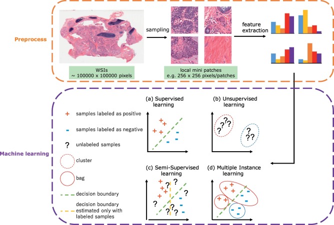
Typical steps for machine learning in digital pathological image analysis.
In this article we will try to apply CNN ResNet architecture to classify tissue types of colon, we will consider patches with different labels such as: mucosa, tumor, stroma, lympho and etc. We won’t consider transfering learning case and will train CNN from scratch because weights from pretrained models were obtained from ImageNet images which is not related to histology field and won’t help in quicker model convergenge.
Dataset
As a dataset I selected collection of textures in colorectal cancer histology, it can be considered as a MNIST for biologists. You can find this dataset at Zenodo or at Kaggle platform
TDAtaset contains two zipped folders:
- “Kather_texture_2016_image_tiles_5000.zip”: a zipped folder containing 5000 histological images of 150 * 150 px each (74 * 74 µm). Each image belongs to exactly one of eight tissue categories (specified by the folder name).
- “Kather_texture_2016_larger_images_10.zip”: a zipped folder containing 10 larger histological images of 5000 x 5000 px each. These images contain more than one tissue type.
All images are RGB, 0.495 µm per pixel, digitized with an Aperio ScanScope (Aperio/Leica biosystems), magnification 20x. Histological samples are fully anonymized images of formalin-fixed paraffin-embedded human colorectal adenocarcinomas (primary tumors) from pathology archive (Institute of Pathology, University Medical Center Mannheim, Heidelberg University, Mannheim, Germany).
Colorectal MNIST images classification with ResNet
![]()
Import necessary libraries and listing input directory with the data to observe folders structure and stored files. To run kernel I used kaggle notebooks, where you can directly import appropriate data without downloading.
In [1]:
import os
import random
import itertools

import numpy as np
import pandas as pd
import matplotlib.pyplot as plt
from sklearn.model_selection import train_test_split
from PIL import Image
from sklearn.metrics import confusion_matrix, classification_report, multilabel_confusion_matrix
import torch
import torch.nn as nn
import torch.utils.data as D
import torch.nn.functional as F

from torchvision import transforms, models

from tqdm import tqdm

import warnings
warnings.filterwarnings('ignore')

torch.cuda.empty_cache()
Helpers
In [2]:
def display_pil_images(
    images,
    labels,
    columns=5, width=20, height=8, max_images=15,
    label_wrap_length=50, label_font_size=8):

    if not images:
        print("No images to display.")
        return

    if len(images) > max_images:
        print(f"Showing {max_images} images of {len(images)}:")
        images=images[0:max_images]

    height = max(height, int(len(images)/columns) * height)
    plt.figure(figsize=(width, height))

    for i, image in enumerate(images):

        plt.subplot(len(images) / columns + 1, columns, i + 1)
        plt.imshow(image)

        plt.title(labels[i], fontsize=label_font_size);

def show_input(input_tensor, title=''):
    image = input_tensor.permute(1, 2, 0).numpy()
    image = std * image + mean
    plt.imshow(image.clip(0, 1))
    plt.title(title)
    plt.show()
    plt.pause(0.001)

def plot_confusion_matrix(cm, classes, normalize=False, title='Confusion matrix', cmap=plt.cm.Blues):
    if normalize:
        cm = cm.astype('float') / cm.sum[axis=1](:, np.newaxis)
        print("Normalized confusion matrix")
    else:
        print('Confusion matrix, without normalization')

    print(cm)
    plt.imshow(cm, interpolation='nearest', cmap=cmap)
    plt.title(title)
    plt.colorbar()
    tick_marks = np.arange(len(classes))
    plt.xticks(tick_marks, classes, rotation=45)
    plt.yticks(tick_marks, classes)

    fmt = '.2f' if normalize else 'd'
    thresh = cm.max() / 2.
    for i, j in itertools.product(range(cm.shape[0]), range(cm.shape[1])):
        plt.text(j, i, format(cm[i, j], fmt), horizontalalignment="center", color="white" if cm[i, j] > thresh else "black")

    plt.tight_layout()
    plt.ylabel('True label')
    plt.xlabel('Predicted label')
We will consider directory with small images 150 x 150 in size. To feed images into ResNet CNN model you need to resize them to 224 x 224 size.
In [3]:
DATA_DIR = '/kaggle/input/colorectal-histology-mnist/'
SMALL_IMG_DATA_DIR = os.path.join(DATA_DIR, 'kather_texture_2016_image_tiles_5000/Kather_texture_2016_image_tiles_5000')
LARGE_IMG_DATA_DIR = os.path.join(DATA_DIR, 'kather_texture_2016_larger_images_10/Kather_texture_2016_larger_images_10')

IMAGE_SIZE = 224
SEED = 2000
BATCH_SIZE = 64
NUM_EPOCHS = 15

random.seed(SEED)
np.random.seed(SEED)
torch.manual_seed(SEED)
torch.cuda.manual_seed(SEED)
torch.backends.cudnn.deterministic = True

device = torch.device("cuda:0" if torch.cuda.is_available() else "cpu")
Data exploration
Here we can see 8 folders with names corresponding to the labels for our model.
In [4]:
classes = os.listdir(SMALL_IMG_DATA_DIR)
classes
['03_COMPLEX',
'08_EMPTY',
'04_LYMPHO',
'01_TUMOR',
'02_STROMA',
'06_MUCOSA',
'05_DEBRIS',
'07_ADIPOSE']
In [5]:
os.listdir(LARGE_IMG_DATA_DIR)['CRC-Prim-HE-05_APPLICATION.tif',
'CRC-Prim-HE-04_APPLICATION.tif',
'CRC-Prim-HE-10_APPLICATION.tif',
'CRC-Prim-HE-06_APPLICATION.tif',
'CRC-Prim-HE-03_APPLICATION.tif',
'CRC-Prim-HE-01_APPLICATION.tif',
'CRC-Prim-HE-08_APPLICATION.tif',
'CRC-Prim-HE-02-APPLICATION.tif',
'CRC-Prim-HE-07_APPLICATION.tif',
'CRC-Prim-HE-09_APPLICATION.tif']
Let’s select random number for each folder to display random samples from input dataset.
In [6]:
samples_to_view = []
for label in classes:
    num_samples = len(os.listdir(os.path.join(SMALL_IMG_DATA_DIR,label)))
    print(label + '\t' + str(num_samples))
    samples_to_view.append(random.choice(np.arange(num_samples)))
03_COMPLEX 625
08_EMPTY 625
04_LYMPHO 625
01_TUMOR 625
02_STROMA 625
06_MUCOSA 625
05_DEBRIS 625
07_ADIPOSE 625
In [7]:
imgs = []
for idx, label in enumerate(classes):
    show_idx = samples_to_view[idx]
    file_name = os.listdir(os.path.join(SMALL_IMG_DATA_DIR,label))[show_idx]
    print(file_name)
    imgs.append(Image.open(os.path.join(SMALL_IMG_DATA_DIR,label,file_name)))
5C8E_CRC-Prim-HE-08_005.tif_901_Col_1.tif
1429C_CRC-Prim-HE-06_005.tif_5401_Col_6451.tif
6408_CRC-Prim-HE-05_004.tif_451_Col_1.tif
154F0_CRC-Prim-HE-09_024.tif_151_Col_151.tif
13F70_CRC-Prim-HE-07_014.tif_751_Col_1351.tif
1754A_CRC-Prim-HE-06_001.tif_601_Col_751.tif
1688C_CRC-Prim-HE-08_023.tif_451_Col_151.tif
16CE8_CRC-Prim-HE-03_012.tif_1801_Col_901.tif
In [8]:
display_pil_images(imgs, classes)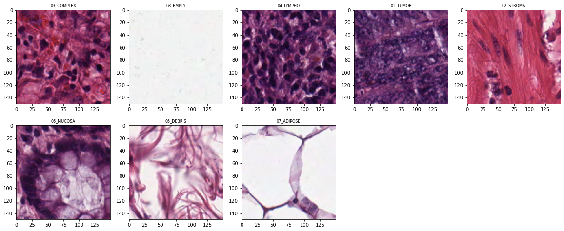
Form DataFrame with image paths and corresponding labels to use in PyTorch Dataset class.
In [9]:
imgs_paths, labels = [], []
for label in classes:
    file_names = os.listdir(os.path.join(SMALL_IMG_DATA_DIR,label))
    for file_name in file_names:
        imgs_paths.append(os.path.join(SMALL_IMG_DATA_DIR,label,file_name))
        labels.append(label)
In [10]:
df = pd.DataFrame(data={'img_path': imgs_paths, 'label': labels})
df.head()| img_path | label | |
|---|---|---|
| 0 | /kaggle/input/colorectal-histology-mnist/kathe... | 03_COMPLEX |
| 1 | /kaggle/input/colorectal-histology-mnist/kathe... | 03_COMPLEX |
| 2 | /kaggle/input/colorectal-histology-mnist/kathe... | 03_COMPLEX |
| 3 | /kaggle/input/colorectal-histology-mnist/kathe... | 03_COMPLEX |
| 4 | /kaggle/input/colorectal-histology-mnist/kathe... | 03_COMPLEX |
Let’s map string label into integer number (label encoding procedure)
In [11]:
label_num = {}
for idx, item in enumerate(np.unique(df.label)):
    label_num[item] = idx
In [12]:
df['label_num'] = df['label'].apply(lambda x: label_num[x])PyTorch Dataset, Dataloaders and Transforms preparation
In [13]:
class HistologyMnistDS(D.Dataset):
    def __init__(self, df, transforms, mode='train'):

        self.records = df.to_records(index=False)
        self.transforms = transforms
        self.mode = mode
        self.len = df.shape[0]

    @staticmethod
    def _load_image_pil(path):
        return Image.open(path)

    def __getitem__(self, index):
        path = self.records[index].img_path

        img = self._load_image_pil(path)

        if self.transforms:
            img = self.transforms(img)

        if self.mode in ['train', 'val', 'test']:
            return img, torch.from_numpy(np.array(self.records[index].label_num))
        else:
            return img

    def __len__(self):
        return self.len
Here is the basic transforms for train, validation and test dataset, but you can add other augmentations to increase variance of the data.
In [14]:
train_transforms = transforms.Compose([
    transforms.Resize((IMAGE_SIZE, IMAGE_SIZE)),
    transforms.ToTensor(),
    transforms.Normalize([0.485, 0.456, 0.406], [0.229, 0.224, 0.225])
])

val_transforms = transforms.Compose([
    transforms.Resize((IMAGE_SIZE, IMAGE_SIZE)),
    transforms.ToTensor(),
    transforms.Normalize([0.485, 0.456, 0.406], [0.229, 0.224, 0.225])
])
Split the data into train, validation and test datasets. Train set usually used to adjust the weights, validation set - for hyperparameters optimization, and test set is for model performance testing.
In [15]:
train_df, tmp_df = train_test_split(df,
                                      test_size=0.2,
                                      random_state=SEED,
                                      stratify=df['label'])

valid_df, test_df = train_test_split(tmp_df,
                                      test_size=0.8,
                                      random_state=SEED,
                                      stratify=tmp_df['label'])
In [16]:
print("Train DF shape:", train_df.shape)
print("Valid DF shape:", valid_df.shape)
print("Test DF shape:", test_df.shape)
Train DF shape: (4000, 3)
Valid DF shape: (200, 3)
Test DF shape: (800, 3)
Create dataset objects and corresponding data loaders
In [17]:
ds_train = HistologyMnistDS(train_df, train_transforms)
ds_val = HistologyMnistDS(valid_df, val_transforms, mode='val')
ds_test = HistologyMnistDS(test_df, val_transforms, mode='test')
In [18]:
train_loader = D.DataLoader(ds_train, batch_size=BATCH_SIZE, shuffle=True, num_workers=4)
val_loader = D.DataLoader(ds_val, batch_size=BATCH_SIZE, shuffle=False, num_workers=4)
test_loader = D.DataLoader(ds_test, batch_size=BATCH_SIZE, shuffle=False, num_workers=4)
In [19]:
X_batch, y_batch = next(iter(train_loader))
mean = np.array([0.485, 0.456, 0.406])
std = np.array([0.229, 0.224, 0.225])
plt.imshow(X_batch[0].permute(1, 2, 0).numpy() * std + mean)
plt.title(y_batch[0]);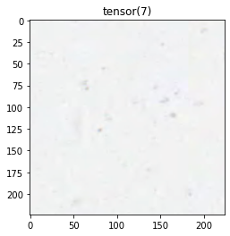
Train loop
In [20]:
import copy

checkpoints_dir = '/kaggle/working/'

history_train_loss, history_val_loss = [], []

def train_model(model, loss, optimizer, scheduler, num_epochs):
    best_model_wts = copy.deepcopy(model.state_dict())

    best_loss = 10e10
    best_acc_score = 0.0

    for epoch in range(num_epochs):
        print('Epoch {}/{}:'.format(epoch, num_epochs - 1), flush=True)

        for phase in ['train', 'val']:
            if phase == 'train':
                dataloader = train_loader
                scheduler.step()
                model.train()
            else:
                dataloader = val_loader
                model.eval()

            running_loss = 0.
            running_acc = 0.

            # Iterate over data.
            for inputs, labels in tqdm(dataloader):
                inputs = inputs.to(device)
                labels = labels.to(device)

                optimizer.zero_grad()

                # forward and backward
                with torch.set_grad_enabled(phase == 'train'):
                    preds = model(inputs)
                    loss_value = loss(preds, labels)
                    preds_class = preds.argmax(dim=1)

                    # backward + optimize only if in training phase
                    if phase == 'train':
                        loss_value.backward()
                        optimizer.step()

                # statistics
                running_loss += loss_value.item()
                running_acc += (preds_class == labels.data).float().mean()

            epoch_loss = running_loss / len(dataloader)
            epoch_acc = running_acc / len(dataloader)

            print('{} Loss: {:.4f} Acc: {:.4f}'.format(phase, epoch_loss, epoch_acc), flush=True)

            if phase == 'train':
                history_train_loss.append(epoch_loss)
            else:
                history_val_loss.append(epoch_loss)

            if phase == 'val':
                def save_checkpoint(name):
                    checkpoint = {
                        'state_dict': best_model_wts
                    }

                    model_file_name = name + '.pth.tar'

                    model_file = checkpoints_dir + model_file_name

                    if not os.path.exists(checkpoints_dir):
                        os.mkdir(checkpoints_dir)

                    # saving best weights of model
                    torch.save(checkpoint, model_file)

                if epoch_loss < best_loss:
                    best_loss = epoch_loss
                    best_model_wts = copy.deepcopy(model.state_dict())
                    print("Saving model for best loss")
                    save_checkpoint('best_model')

                if epoch_acc > best_acc_score:
                    best_acc_score = epoch_acc

                print('Best_loss: {:.4f}'.format(best_loss))
                print('Best_acc_score: {:.4f}'.format(best_acc_score))

    return model
Model setup and training
Here ResNet model with 50 layers is used, we replace last linear layer to satisfy the requirement for number of classes. Additionally linear scheduler is used and will reduce learning rate of Adam optimizer every 7 epochs.
In [21]:
model = models.resnet50(pretrained=False)

model.fc = torch.nn.Linear(model.fc.in_features, len(classes))
model = model.to(device)

loss = torch.nn.CrossEntropyLoss()
optimizer = torch.optim.Adam(model.parameters(), lr=1.0e-3)
scheduler = torch.optim.lr_scheduler.StepLR(optimizer, step_size=7, gamma=0.1)
In [22]:
train_model(model, loss, optimizer, scheduler, num_epochs=NUM_EPOCHS);Epoch 0/9:
100%|██████████| 63/63 [00:25<00:00, 2.46it/s]
train Loss: 1.0313 Acc: 0.6414
100%|██████████| 4/4 [00:01<00:00, 3.25it/s]
val Loss: 0.7102 Acc: 0.7578
Saving model for best loss
Best_loss: 0.7102
Best_acc_score: 0.7578
Epoch 1/9:
100%|██████████| 63/63 [00:26<00:00, 2.42it/s]
train Loss: 0.6983 Acc: 0.7587
100%|██████████| 4/4 [00:01<00:00, 3.25it/s]
val Loss: 4.5117 Acc: 0.6250
Best_loss: 0.7102
Best_acc_score: 0.7578
Epoch 2/9:
100%|██████████| 63/63 [00:25<00:00, 2.45it/s]
train Loss: 0.6180 Acc: 0.7862
100%|██████████| 4/4 [00:01<00:00, 3.40it/s]
val Loss: 0.4103 Acc: 0.8477
Saving model for best loss
Best_loss: 0.4103
Best_acc_score: 0.8477
Epoch 3/9:
100%|██████████| 63/63 [00:25<00:00, 2.43it/s]
train Loss: 0.5134 Acc: 0.8209
100%|██████████| 4/4 [00:01<00:00, 3.32it/s]
val Loss: 0.3510 Acc: 0.8516
Saving model for best loss
Best_loss: 0.3510
Best_acc_score: 0.8516
Epoch 4/9:
100%|██████████| 63/63 [00:25<00:00, 2.47it/s]
train Loss: 0.4767 Acc: 0.8182
100%|██████████| 4/4 [00:01<00:00, 3.18it/s]
val Loss: 2.5895 Acc: 0.6641
Best_loss: 0.3510
Best_acc_score: 0.8516
Epoch 5/9:
100%|██████████| 63/63 [00:25<00:00, 2.46it/s]
train Loss: 0.4765 Acc: 0.8259
100%|██████████| 4/4 [00:01<00:00, 3.25it/s]
val Loss: 0.4351 Acc: 0.8398
Best_loss: 0.3510
Best_acc_score: 0.8516
Epoch 6/9:
100%|██████████| 63/63 [00:26<00:00, 2.42it/s]
train Loss: 0.3701 Acc: 0.8676
100%|██████████| 4/4 [00:01<00:00, 3.34it/s]
val Loss: 0.1979 Acc: 0.9414
Saving model for best loss
Best_loss: 0.1979
Best_acc_score: 0.9414
Epoch 7/9:
100%|██████████| 63/63 [00:25<00:00, 2.45it/s]
train Loss: 0.3140 Acc: 0.8886
100%|██████████| 4/4 [00:01<00:00, 3.49it/s]
val Loss: 0.1852 Acc: 0.9414
Saving model for best loss
Best_loss: 0.1852
Best_acc_score: 0.9414
Epoch 8/9:
100%|██████████| 63/63 [00:26<00:00, 2.42it/s]
train Loss: 0.2892 Acc: 0.9000
100%|██████████| 4/4 [00:01<00:00, 3.30it/s]
val Loss: 0.1873 Acc: 0.9375
Best_loss: 0.1852
Best_acc_score: 0.9414
Epoch 9/9:
100%|██████████| 63/63 [00:25<00:00, 2.45it/s]
train Loss: 0.2876 Acc: 0.9015
100%|██████████| 4/4 [00:01<00:00, 2.71it/s]
val Loss: 0.1765 Acc: 0.9414
Saving model for best loss
Best_loss: 0.1765
Best_acc_score: 0.9414
Validation and test results
We can see that our model quickly converged to a good results.
In [23]:
x = np.arange(NUM_EPOCHS)
plt.plot(x, history_train_loss)
plt.plot(x, history_val_loss)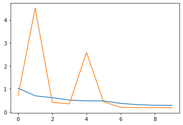
In [24]:
filename = "best_model.pth.tar"

model.load_state_dict(torch.load(os.path.join(checkpoints_dir, filename))['state_dict'])

model.eval()

y_preds = []
for inputs, labels in tqdm(test_loader):
    inputs = inputs.to(device)
    labels = labels.to(device)
    with torch.set_grad_enabled(False):
        preds = model(inputs)
    y_preds.append(preds.argmax(dim=1).data.cpu().numpy())

y_preds = np.concatenate(y_preds)
100%|██████████| 13/13 [00:04<00:00, 3.17it/s]
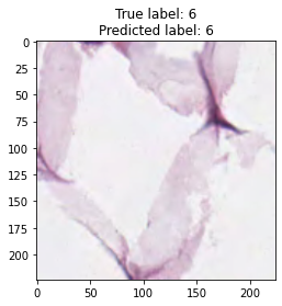
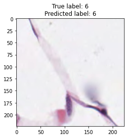
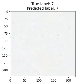
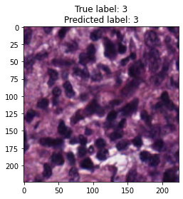
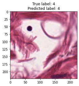
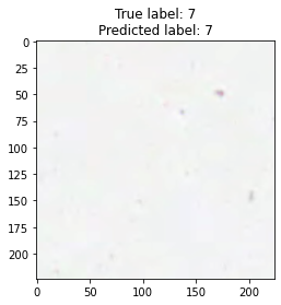
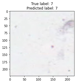
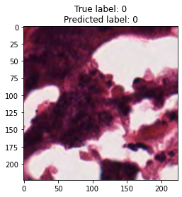
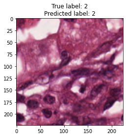
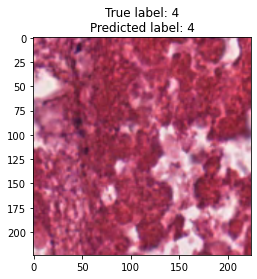
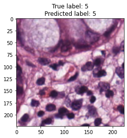
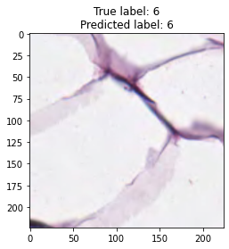
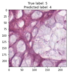
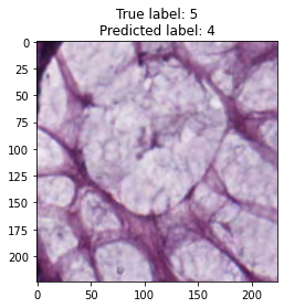
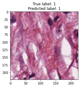
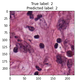
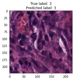
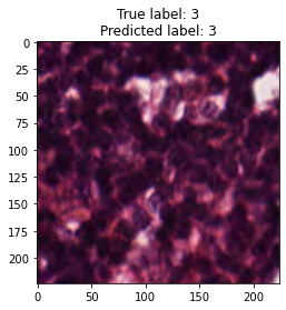
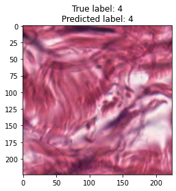
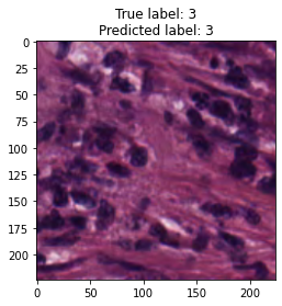
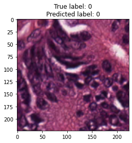
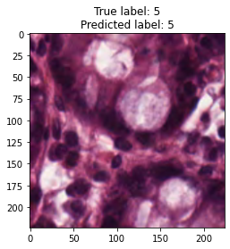
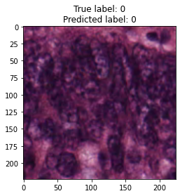
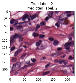
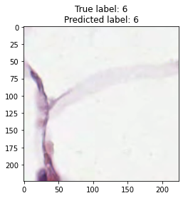
In [25]:
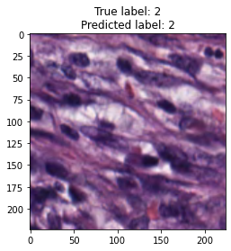
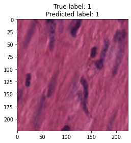
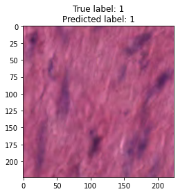
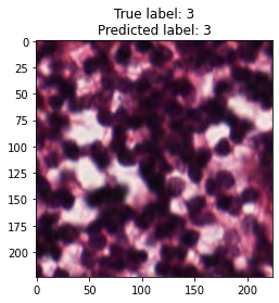
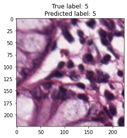
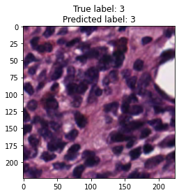
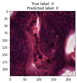
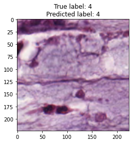
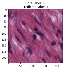
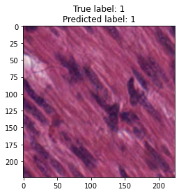
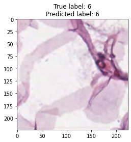
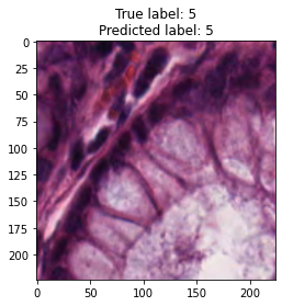
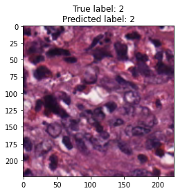
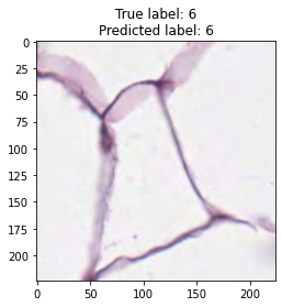
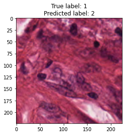
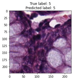
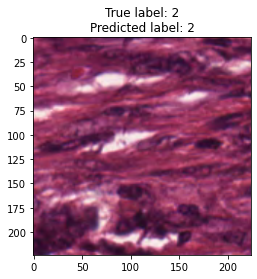
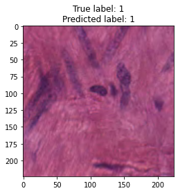
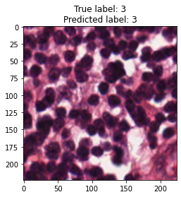
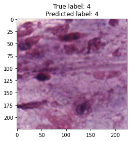
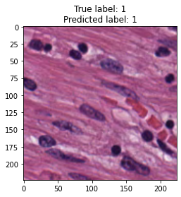
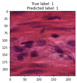
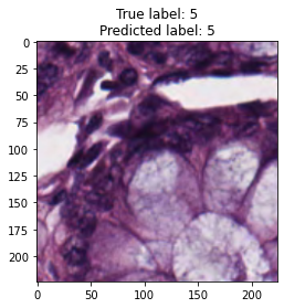
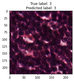
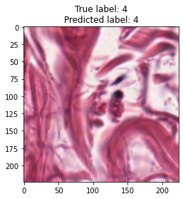
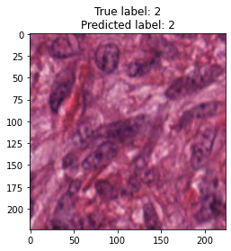
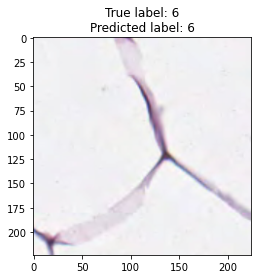
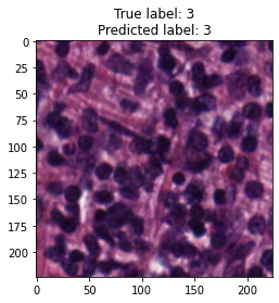
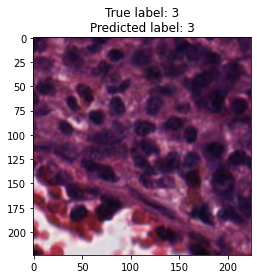
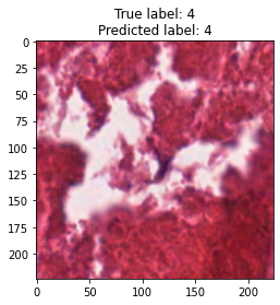
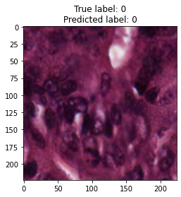
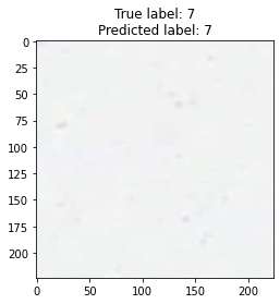
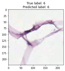
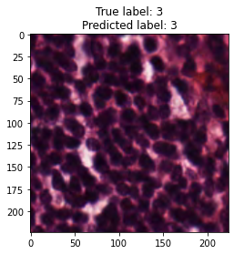
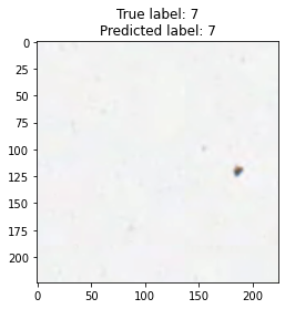
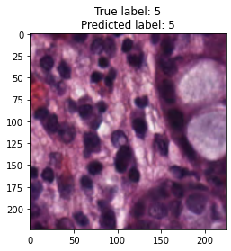
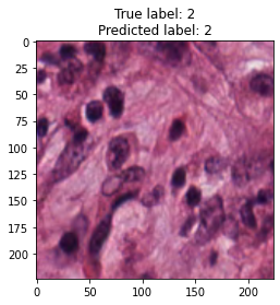
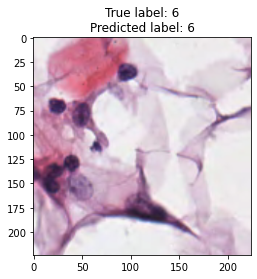
inputs, labels = next(iter(test_loader))

for img, label, pred in zip(inputs, labels, y_preds):
    title = f"True label: {label}\nPredicted label: {pred}"
    show_input(img, title=title)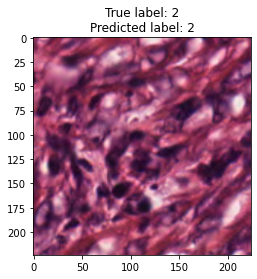
In [26]:
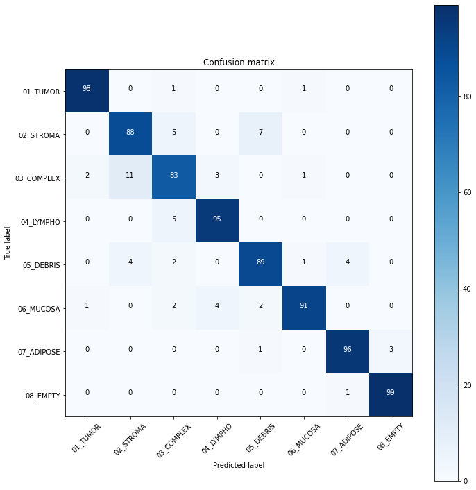
cm = confusion_matrix(test_df.label_num.values, y_preds)In [27]:
plt.figure(figsize=(10,10))
plot_confusion_matrix(cm, label_num)
Confusion matrix, without normalization
[[98 0 1 0 0 1 0 0]
[ 0 88 5 0 7 0 0 0]
[ 2 11 83 3 0 1 0 0]
[ 0 0 5 95 0 0 0 0]
[ 0 4 2 0 89 1 4 0]
[ 1 0 2 4 2 91 0 0]
[ 0 0 0 0 1 0 96 3]
[ 0 0 0 0 0 0 1 99]]
In [28]:
print(classification_report(test_df.label_num.values,
                            y_preds,
                            target_names=list(label_num.keys())))
precision recall f1-score support
01_TUMOR 0.97 0.98 0.98 100
02_STROMA 0.85 0.88 0.87 100
03_COMPLEX 0.85 0.83 0.84 100
04_LYMPHO 0.93 0.95 0.94 100
05_DEBRIS 0.90 0.89 0.89 100
06_MUCOSA 0.97 0.91 0.94 100
07_ADIPOSE 0.95 0.96 0.96 100
08_EMPTY 0.97 0.99 0.98 100
accuracy 0.92 800
macro avg 0.92 0.92 0.92 800
weighted avg 0.92 0.92 0.92 800
Conclusion
We trained the ResNet-50 model for 15 epochs, although the model showed good accuracy. From model results on test dataset we can see that tumor and empty are recognizable with f1 score equal to 0.98, the most confusable label is complex which probably represents combinations of other tissue types.