This tutorial contains brief overview of statistical and machine learning methods for time series forecasting, experiments and comparative analysis of Long short-term memory (LSTM) based architectures for solving above mentioned problem. Single layer, two layer and bidirectional single layer LSTM cases are considered. Metro Interstate Traffic Volume Data Set from UCI Machine Learning Repository and PyTorch deep learning framework are used for analysis.

• Time series forecasting methods overview
• Dataset
• Metro Traffic Prediction using LSTM-based recurrent neural network
  • Exploratory Data Analysis (EDA) and Scaling
  • Preparing training dataset/Visualizations
  • LSTM Time Series Predictor Model
  • Train and Evaluate Helping Functions
  • 1-Layer LSTM model
  • 2-Layer LSTM
  • Bidirectional 1-Layer LSTM
  • Experimental results on val data
• Summary

Time series forecasting methods overview

A time series is a set of observations, each one is being recorded at the specific time \(t\). It can be weather observations, for example, a records of the temperature for a month, it can be observations of currency quotes during the day or any other process aggregated by time. Time series forecasting can be determened as the act of predicting the future by understanding the past. The model for forecasting can rely on one variable and this is a univariate case or when more than one variable taken into consideration it will be multivariate case.

Stochastic Linear Models:

• Autoregressive (AR);
• Moving Average (MA);
• Autoregressive Moving Average (ARMA);
• Autoregressive Integrated Moving Average (ARIMA);
• Seasonal ARIMA (SARIMA).

For above family of models, the stationarity condition must be satisfied. Loosely speaking, a stochastic process is stationary, if its statistical properties do not change with time.

Stochastic Non-Linear Models:

• nonlinear autoregressive exogenous models (NARX);
• autoregressive conditional heteroskedasticity (ARCH);
• generalized autoregressive conditional heteroskedasticity (GARCH).

Machine Learning Models

• Hidden Markov Model;
• Least-square SVM (LS-SVM);
• Dynamic Least-square SVM (DLS-SVM);
• Feed Forward Network (FNN);
• Time Lagged Neural Network (TLNN);
• Seasonal Artificial Neural Network (SANN);
• Recurrent Neural Networks (RNN).

Dataset

We will use Metro Interstate Traffic Volume Data Set from UC Irvine Machine Learning Repository, which contains large number of datasets for various tasks in machine learning. We will investigate how weather and holiday features influence the metro traffic in US.

Attribute Information:

holiday Categorical US National holidays plus regional holiday, Minnesota State;
temp Numeric Average temp in kelvin;
rain_1h Numeric Amount in mm of rain that occurred in the hour;
snow_1h Numeric Amount in mm of snow that occurred in the hour;
clouds_all Numeric Percentage of cloud cover;
weather_main Categorical Short textual description of the current weather;
weather_description Categorical Longer textual description of the current weather;
date_time DateTime Hour of the data collected in local CST time;
traffic_volume Numeric Hourly I-94 ATR 301 reported westbound traffic volume.

Our target variable will be traffic_volume. Here we will consider multivariate multi-step prediction case with LSTM-based recurrent neural network architecture.

Metro Traffic Prediction using LSTM-based recurrent neural network

I used Google Colab Notebooks to calculate experiments. Here, for convinience, I mounted my Google drive where I stored the files.

In [1]:

from google.colab import drive
drive.mount('/content/drive', force_remount=True)

Out [1]:

Mounted at /content/drive

In [2]:

import os
import copy
import random
import numpy as np
import pandas as pd
import matplotlib.pyplot as plt

import torch
import torch.nn as nn
from torch.autograd import Variable

import warnings
warnings.filterwarnings('ignore')

In [3]:

random.seed(0)
np.random.seed(0)
torch.manual_seed(0)
torch.cuda.manual_seed(0)
torch.backends.cudnn.deterministic = True

In [4]:

data = pd.read_csv('/content/drive/My Drive/time series prediction/Metro_Interstate_Traffic_Volume.csv', parse_dates=True)

Exploratory Data Analysis (EDA) and Scaling

In [5]:

data.head()

Out [5]:

	holiday	temp	rain_1h	snow_1h	clouds_all	weather_main	weather_description	date_time	traffic_volume
0	None	288.28	0.0	0.0	40	Clouds	scattered clouds	2012-10-02 09:00:00	5545
1	None	289.36	0.0	0.0	75	Clouds	broken clouds	2012-10-02 10:00:00	4516
2	None	289.58	0.0	0.0	90	Clouds	overcast clouds	2012-10-02 11:00:00	4767
3	None	290.13	0.0	0.0	90	Clouds	overcast clouds	2012-10-02 12:00:00	5026
4	None	291.14	0.0	0.0	75	Clouds	broken clouds	2012-10-02 13:00:00	4918

categorical features: holiday, weather_main, weather_description.
Continious features: temp, rain_1h, show_1h, clouds_all.
Target variable: traffic_volume

In [6]:

data.info()

Out [6]:

<class 'pandas.core.frame.DataFrame'>
RangeIndex: 48204 entries, 0 to 48203
Data columns (total 9 columns):
 #   Column               Non-Null Count  Dtype  
---  ------               --------------  -----  
 0   holiday              48204 non-null  object 
 1   temp                 48204 non-null  float64
 2   rain_1h              48204 non-null  float64
 3   snow_1h              48204 non-null  float64
 4   clouds_all           48204 non-null  int64  
 5   weather_main         48204 non-null  object 
 6   weather_description  48204 non-null  object 
 7   date_time            48204 non-null  object 
 8   traffic_volume       48204 non-null  int64  
dtypes: float64(3), int64(2), object(4)
memory usage: 3.3+ MB

Checking for Nan values

In [7]:

for column in data.columns:
    print(column, sum(data[column].isna()))

Out [7]:

holiday 0
temp 0
rain_1h 0
snow_1h 0
clouds_all 0
weather_main 0
weather_description 0
date_time 0
traffic_volume 0

Here I take into consideration two categorical variables, such as ‘holiday’ and ‘weather_main’ and then one-hot encode them.

In [8]:

data = pd.get_dummies(data, columns = ['holiday', 'weather_main'], drop_first=True)

In [9]:

data.head()

Out [9]:

	temp	rain_1h	snow_1h	clouds_all	weather_description	date_time	traffic_volume	holiday_Columbus Day	holiday_Independence Day	holiday_Labor Day	holiday_Martin Luther King Jr Day	holiday_Memorial Day	holiday_New Years Day	holiday_None	holiday_State Fair	holiday_Thanksgiving Day	holiday_Veterans Day	holiday_Washingtons Birthday	weather_main_Clouds	weather_main_Drizzle	weather_main_Fog	weather_main_Haze	weather_main_Mist	weather_main_Rain	weather_main_Smoke	weather_main_Snow	weather_main_Squall	weather_main_Thunderstorm
0	288.28	0.0	0.0	40	scattered clouds	2012-10-02 09:00:00	5545	0	0	0	0	0	0	1	0	0	0	0	1	0	0	0	0	0	0	0	0	0
1	289.36	0.0	0.0	75	broken clouds	2012-10-02 10:00:00	4516	0	0	0	0	0	0	1	0	0	0	0	1	0	0	0	0	0	0	0	0	0
2	289.58	0.0	0.0	90	overcast clouds	2012-10-02 11:00:00	4767	0	0	0	0	0	0	1	0	0	0	0	1	0	0	0	0	0	0	0	0	0
3	290.13	0.0	0.0	90	overcast clouds	2012-10-02 12:00:00	5026	0	0	0	0	0	0	1	0	0	0	0	1	0	0	0	0	0	0	0	0	0
4	291.14	0.0	0.0	75	broken clouds	2012-10-02 13:00:00	4918	0	0	0	0	0	0	1	0	0	0	0	1	0	0	0	0	0	0	0	0	0

In [10]:

data.shape

Out [10]:

(48204, 28)

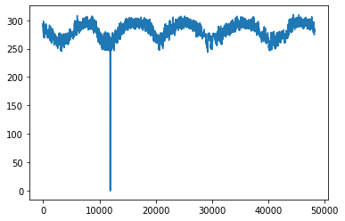
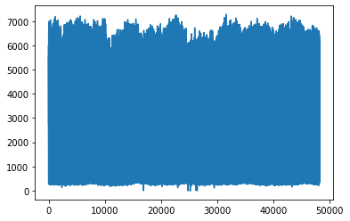
Here we can see outliers in ‘temp’ variable, lets filter outliers with Interquartile range (IQR) method

In [11]:

data['temp'].plot()
plt.show()
data['traffic_volume'].plot()
plt.show()

Out [11]:

In [12]:

Q1 = data.quantile(0.25)
Q3 = data.quantile(0.75)
IQR = Q3 - Q1
print(IQR)

Out [12]:

temp                                   19.646
rain_1h                                 0.000
snow_1h                                 0.000
clouds_all                             89.000
traffic_volume                       3740.000
holiday_Columbus Day                    0.000
holiday_Independence Day                0.000
holiday_Labor Day                       0.000
holiday_Martin Luther King Jr Day       0.000
holiday_Memorial Day                    0.000
holiday_New Years Day                   0.000
holiday_None                            0.000
holiday_State Fair                      0.000
holiday_Thanksgiving Day                0.000
holiday_Veterans Day                    0.000
holiday_Washingtons Birthday            0.000
weather_main_Clouds                     1.000
weather_main_Drizzle                    0.000
weather_main_Fog                        0.000
weather_main_Haze                       0.000
weather_main_Mist                       0.000
weather_main_Rain                       0.000
weather_main_Smoke                      0.000
weather_main_Snow                       0.000
weather_main_Squall                     0.000
weather_main_Thunderstorm               0.000
dtype: float64

In [13]:

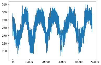
data = data[~((data['temp'] < (Q1['temp'] - 1.5 * IQR['temp'])) |(data['temp'] > (Q3['temp'] + 1.5 * IQR['temp'])))]

In [14]:

data['temp'].plot()
plt.show()
data['traffic_volume'].plot()
plt.show()

Out [14]:

In [15]:

 data.drop(columns=['rain_1h', 'snow_1h', 'weather_description', 'date_time'], inplace=True)

Normalizing the features

In [16]:

features_to_norm = ['temp', 'clouds_all', 'traffic_volume']

In [17]:

TRAIN_SPLIT = 40000
STEP = 6

past_history = 720
future_target = 32
target_index = 2

tmp = data[features_to_norm].values
data_mean = tmp[:TRAIN_SPLIT].mean(axis=0)
data_std = tmp[:TRAIN_SPLIT].std(axis=0)

In [18]:

data[features_to_norm] = (data[features_to_norm]-data_mean)/data_std

In [19]:

data

Out [19]:

	temp	clouds_all	traffic_volume	holiday_Columbus Day	holiday_Independence Day	holiday_Labor Day	holiday_Martin Luther King Jr Day	holiday_Memorial Day	holiday_New Years Day	holiday_None	holiday_State Fair	holiday_Thanksgiving Day	holiday_Veterans Day	holiday_Washingtons Birthday	weather_main_Clouds	weather_main_Drizzle	weather_main_Fog	weather_main_Haze	weather_main_Mist	weather_main_Rain	weather_main_Smoke	weather_main_Snow	weather_main_Squall	weather_main_Thunderstorm
0	0.581321	-0.261692	1.145383	0	0	0	0	0	0	1	0	0	0	0	1	0	0	0	0	0	0	0	0	0
1	0.668789	0.638749	0.628729	0	0	0	0	0	0	1	0	0	0	0	1	0	0	0	0	0	0	0	0	0
2	0.686606	1.024652	0.754754	0	0	0	0	0	0	1	0	0	0	0	1	0	0	0	0	0	0	0	0	0
3	0.731150	1.024652	0.884797	0	0	0	0	0	0	1	0	0	0	0	1	0	0	0	0	0	0	0	0	0
4	0.812948	0.638749	0.830570	0	0	0	0	0	0	1	0	0	0	0	1	0	0	0	0	0	0	0	0	0
...	...	...	...	...	...	...	...	...	...	...	...	...	...	...	...	...	...	...	...	...	...	...	...	...
48199	0.190147	0.638749	0.140191	0	0	0	0	0	0	1	0	0	0	0	1	0	0	0	0	0	0	0	0	0
48200	0.134265	1.024652	-0.242404	0	0	0	0	0	0	1	0	0	0	0	1	0	0	0	0	0	0	0	0	0
48201	0.131835	1.024652	-0.554707	0	0	0	0	0	0	1	0	0	0	0	0	0	0	0	0	0	0	0	0	1
48202	0.080003	1.024652	-0.910691	0	0	0	0	0	0	1	0	0	0	0	1	0	0	0	0	0	0	0	0	0
48203	0.082432	1.024652	-1.159730	0	0	0	0	0	0	1	0	0	0	0	1	0	0	0	0	0	0	0	0	0

48194 rows × 24 columns

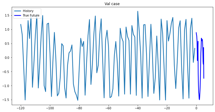
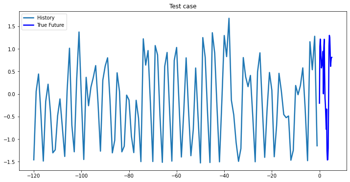
Preparing training dataset/Visualizations

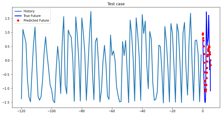
Here we will consider multiple future points prediction case given a past history.

In [20]:

def multivariate_data(dataset, target, start_index, end_index, history_size,
                      target_size, step, single_step=False):
    data = []
    labels = []

    start_index = start_index + history_size
    if end_index is None:
        end_index = len(dataset) - target_size

    for i in range(start_index, end_index):
        indices = range(i-history_size, i, step)
        data.append(dataset[indices])

        if single_step:
            labels.append(target[i+target_size])
        else:
            labels.append(target[i:i+target_size])

    return np.array(data), np.array(labels)

In [21]:

trainX, trainY = multivariate_data(data.values, data.iloc[:, target_index].values, 0,
                                   TRAIN_SPLIT, past_history,
                                   future_target, STEP)

valX, valY = multivariate_data(data.values, data.iloc[:, target_index].values,
                               TRAIN_SPLIT, None, past_history,
                               future_target, STEP)

In [22]:

testX, testY = valX[:len(valX)//4], valY[:len(valY)//4]
valX, valY = valX[len(valX)//4:], valY[len(valY)//4:]

In [23]:

print('Train input features shape : {}'.format(trainX.shape))
print('\nTrain output shape : {}'.format(trainY.shape))
print('\nValidation input features shape : {}'.format(valX.shape))
print('\nValidation output shape : {}'.format(valY.shape))
print('\nTest input features shape : {}'.format(testX.shape))
print('\nTest output shape : {}'.format(testY.shape))

Out [23]:

Train input features shape : (39280, 120, 24)

Train output shape : (39280, 32)

Validation input features shape : (5582, 120, 24)

Validation output shape : (5582, 32)

Test input features shape : (1860, 120, 24)

Test output shape : (1860, 32)

In [24]:

def create_time_steps(length):
    return list(range(-length, 0))

def multi_step_plot(history, true_future, prediction, pic_name):
    plt.figure(figsize=(12, 6))
    num_in = create_time_steps(len(history))
    num_out = len(true_future)

    plt.plot(num_in, np.array(history), label='History', linewidth=2.5)
    plt.plot(np.arange(num_out)/STEP, np.array(true_future), 'b', label='True Future', linewidth=2.5)
    if prediction.any():
        plt.plot(np.arange(num_out)/STEP, np.array(prediction), 'ro', label='Predicted Future', linewidth=2.5)
    plt.legend(loc='upper left')
    plt.title(pic_name)
    plt.show()

multi_step_plot(trainX[0,:,target_index], trainY[0,:], np.array([0]), 'Train case')
multi_step_plot(valX[0,:,target_index], valY[0,:], np.array([0]), 'Val case')
multi_step_plot(testX[0,:,target_index], testY[0,:], np.array([0]), 'Test case')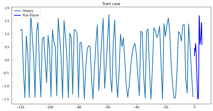

Out [24]:

LSTM Time Series Predictor Model

For more efficient storing of long sequences, here I chose the LSTM architecture. LSTM layer consists from cells which is shown below. Two vectors are inputs to the LSTM-cell: the new input vector from the data \(x_t\) and the vector of the hidden state \(h_{t-1}\), which is obtained from the hidden state of this cell in the previous time step. The LSTM-cell consists of several number of gates and in addition to the hidden state vector, there is a “memory vector” or cell state \(C_t\).
Cell state on time step t is a linear combination of cell state on t-1 time step \(C_{t-1}\) with coefficients from forget gate and new candidate cell state \(\tilde{C_t}\) with coefficients from input gate. When values of forget gate \(f_t\) wiil be close to zero, cell state \(C_{t-1}\) will be forgotten. Where values of input gate vector will be large, the new input vector will be added to that which already were in memory.

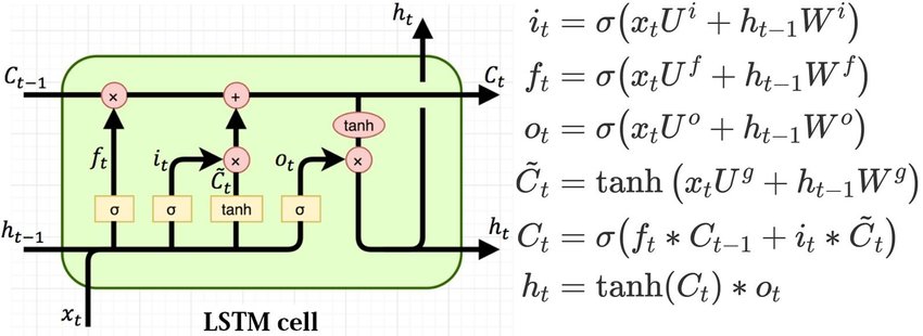
where,
\(i_t\) - input gate;
\(f_t\) - forget gate;
\(o_t\) - output gate;
\(\tilde{C_t}\) - new candidate cell state;
\(C_t\) - cell state;
\(h_t\) - block output.

Peepholes are often added to LSTM cells to increase model connectivity.

In [25]:

class LSTMTimeSeriesPredictor(nn.Module):

    def __init__(self,
                 num_classes,
                 n_features,
                 hidden_size,
                 num_layers,
                 bidirectional=False,
                 dp_rate=0.5):

        super(LSTMTimeSeriesPredictor, self).__init__()

        self.num_layers = num_layers
        self.hidden_size = hidden_size
        self.bidirectional = bidirectional

        self.lstm = nn.LSTM(input_size=n_features,
                            hidden_size=hidden_size,
                            num_layers=num_layers,
                            dropout=dp_rate,
                            batch_first=True,
                            bidirectional=self.bidirectional)

        self.fc = nn.Linear(in_features=hidden_size, out_features=num_classes)

    def forward(self, x):
       # dim(x) = (batch, seq_len, input_size)
       # dim(h_0) = (num_layers *num_directions, batch, hidden_size)
        if self.bidirectional:
            h_0 = Variable(torch.zeros(self.num_layers*2, x.size(0), self.hidden_size))
            c_0 = Variable(torch.zeros(self.num_layers*2, x.size(0), self.hidden_size))
        else:
            h_0 = Variable(torch.zeros(self.num_layers, x.size(0), self.hidden_size))
            c_0 = Variable(torch.zeros(self.num_layers, x.size(0), self.hidden_size))

        o, (h_out,_) = self.lstm(x, (h_0, c_0))

        if self.bidirectional:
            h_out = h_out.view(self.num_layers, 2, x.size(0), self.hidden_size)
            # taking last hidden state
            # dim(h_out) = (num_directions, batch, hidden_size)
            h_out = h_out[-1]

        # in bidectional case we sum vectors over num_directions
        # in the case of multi-layer LSTM we sum over num_layers direction
        # dim(h_out) = (batch, hidden_size)
        h_out = h_out.sum(dim=0)

        # dim(out) = (batch, num_classes)
        out = self.fc(h_out)
        return out

In [26]:

trainX = torch.from_numpy(trainX).float()
trainY = torch.from_numpy(trainY).float()
valX = torch.from_numpy(valX).float()
valY = torch.from_numpy(valY).float()
testX = torch.from_numpy(testX).float()
testY = torch.from_numpy(testY).float()

In [27]:

train_data = torch.utils.data.TensorDataset(trainX, trainY)
val_data = torch.utils.data.TensorDataset(valX, valY)
test_data =  torch.utils.data.TensorDataset(testX, testY)

Train and Evaluate Helping Functions

In [28]:

def train_model(model, train_data, loss_criterion, optimizer, batch_size):

    running_loss = 0.
    model.train()

    train_loader = torch.utils.data.DataLoader(train_data,
                                              batch_size=batch_size,
                                              shuffle=True,
                                              num_workers=0)

    for batch_x, batch_y in train_loader:
        optimizer.zero_grad()

        outputs = model(batch_x)

        loss = loss_criterion(outputs, batch_y)

        loss.backward()

        optimizer.step()

        running_loss += loss.item()

    epoch_loss = running_loss / (len(train_data) // batch_size)

    print("Epoch: %d, train loss: %1.5f" % (epoch+1, epoch_loss))

    return model, epoch_loss

In [29]:

def evaluate_model(model, val_data, loss_criterion, optimizer, batch_size):
    running_loss = 0.
    model.eval()

    val_loader = torch.utils.data.DataLoader(val_data,
                                             batch_size=batch_size,
                                             shuffle=True,
                                             num_workers=0)

    for batch_x, batch_y in val_loader:

        optimizer.zero_grad()

        with torch.set_grad_enabled(False):
            outputs = model(batch_x)
            loss = loss_criterion(outputs, batch_y)

        running_loss += loss.item()

    epoch_loss = running_loss / (len(val_data) // batch_size)

    print("Epoch: %d, val loss: %1.5f" % (epoch+1, epoch_loss))

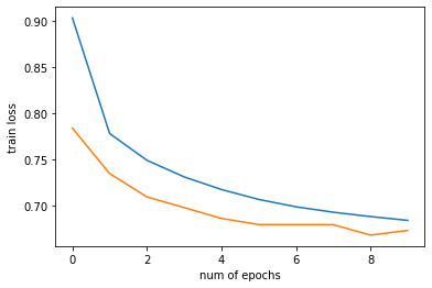
    return model, epoch_loss, best_model_wts

1-Layer LSTM model

In [30]:

learning_rate = 0.001
input_size = trainX.shape[2] # number of input features, multivariate case
hidden_size = 20
num_layers = 1
num_classes = trainY.shape[1] # future time window length
lstm_model = LSTMTimeSeriesPredictor(num_classes, input_size, hidden_size, num_layers, bidirectional=False)

config = {'batch_size': 128, 'num_epochs': 10, 'checkpoints_dir': '/content/drive/My Drive/time series prediction/', 'model_filename': '1-layer-lstm-best_model.pth.tar'}

criterion = torch.nn.MSELoss()
optimizer = torch.optim.Adam(lstm_model.parameters(), lr=learning_rate)

train_history, val_history = [], []

best_model_wts = copy.deepcopy(lstm_model.state_dict())

best_loss = 10e10  # for validation phase

if not os.path.exists(config['checkpoints_dir']):
    os.mkdir(config['checkpoints_dir'])

for epoch in range(config['num_epochs']):
    print("="*20 + str(epoch+1) + "="*20)
    _, train_loss = train_model(lstm_model, train_data, criterion, optimizer, config['batch_size'])
    train_history.append(train_loss)

    _, val_loss, best_model_wts = evaluate_model(lstm_model, val_data, criterion, optimizer, config['batch_size'])
    val_history.append(val_loss)

    if val_loss < best_loss:
        best_loss = val_loss
        print("Saving model for best loss")
        checkpoint = {
            'state_dict': best_model_wts
        }
        torch.save(checkpoint, config['checkpoints_dir'] + config['model_filename'])
        best_model_wts = copy.deepcopy(lstm_model.state_dict())

Out [30]:

====================1====================
Epoch: 1, train loss: 0.90311
Epoch: 1, val loss: 0.78379
Saving model for best loss
====================2====================
Epoch: 2, train loss: 0.77797
Epoch: 2, val loss: 0.73462
Saving model for best loss
====================3====================
Epoch: 3, train loss: 0.74900
Epoch: 3, val loss: 0.70943
Saving model for best loss
====================4====================
Epoch: 4, train loss: 0.73103
Epoch: 4, val loss: 0.69784
Saving model for best loss
====================5====================
Epoch: 5, train loss: 0.71739
Epoch: 5, val loss: 0.68612
Saving model for best loss
====================6====================
Epoch: 6, train loss: 0.70665
Epoch: 6, val loss: 0.67945
Saving model for best loss
====================7====================
Epoch: 7, train loss: 0.69868
Epoch: 7, val loss: 0.67938
Saving model for best loss
====================8====================
Epoch: 8, train loss: 0.69284
Epoch: 8, val loss: 0.67938
====================9====================
Epoch: 9, train loss: 0.68811
Epoch: 9, val loss: 0.66802
Saving model for best loss
====================10====================
Epoch: 10, train loss: 0.68397
Epoch: 10, val loss: 0.67317

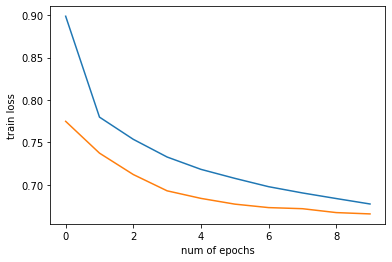
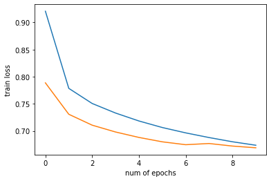
In [31]:

plt.plot(np.arange(config['num_epochs']), train_history, label='Train loss')
plt.plot(np.arange(config['num_epochs']), val_history, label='Val loss')
plt.xlabel("num of epochs")
plt.ylabel("train loss")
plt.show()

Out [31]:

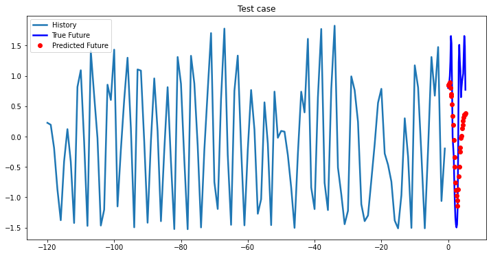
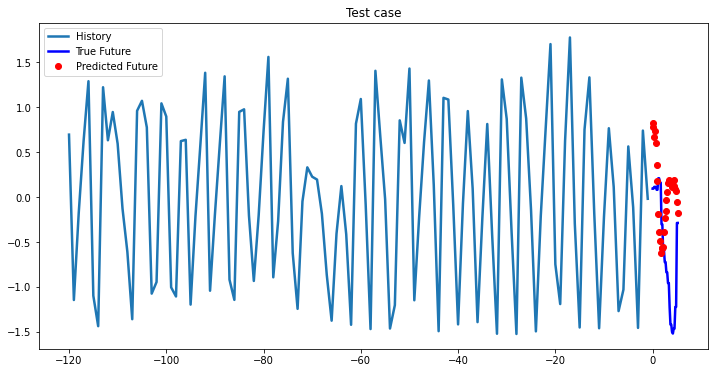
Test

In [32]:

lstm_model = LSTMTimeSeriesPredictor(num_classes, input_size, hidden_size, num_layers)
lstm_model.load_state_dict(torch.load(os.path.join(config['checkpoints_dir'], config['model_filename']))['state_dict'])
lstm_model.eval()
for param in lstm_model.parameters():
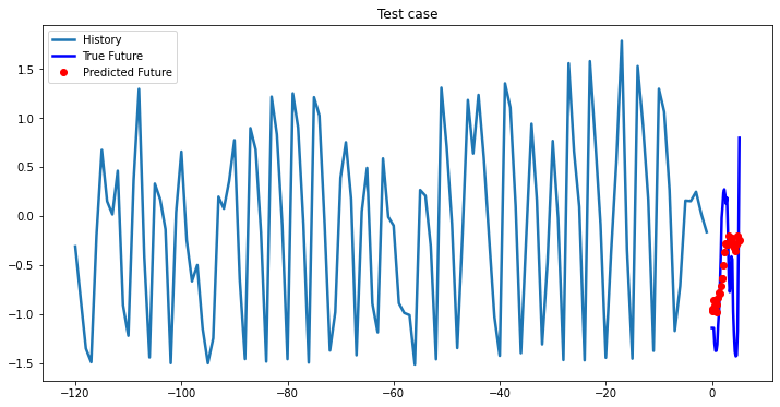
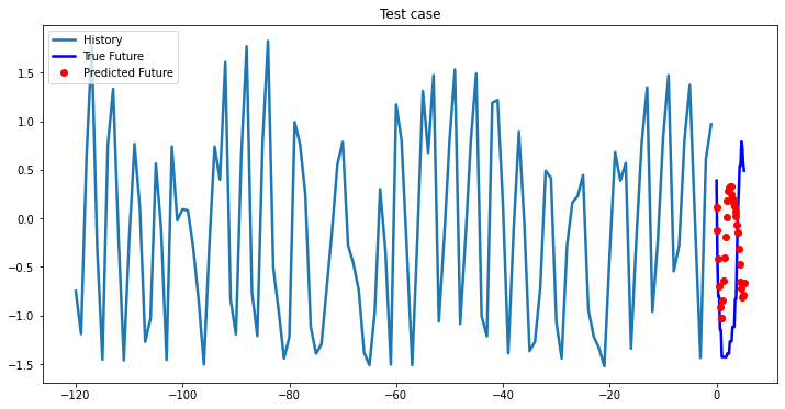
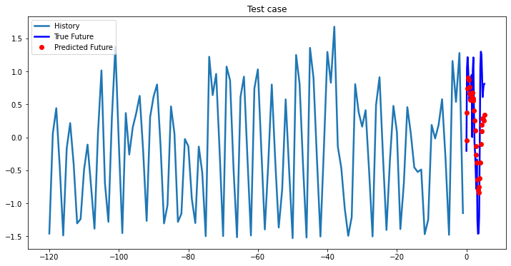
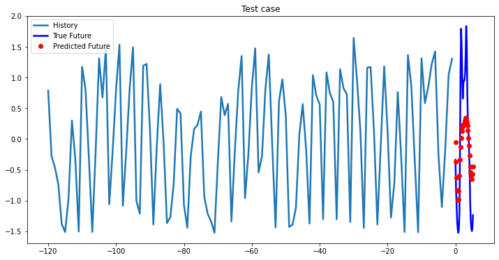
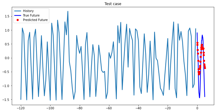
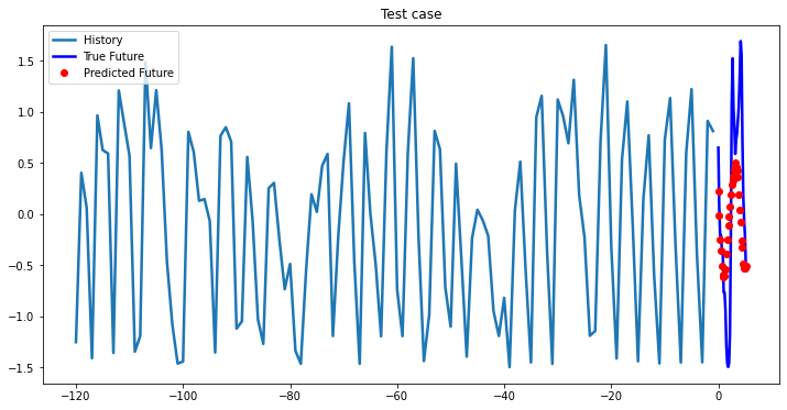
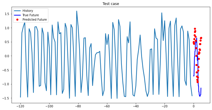
    param.requires_grad = False

In [33]:

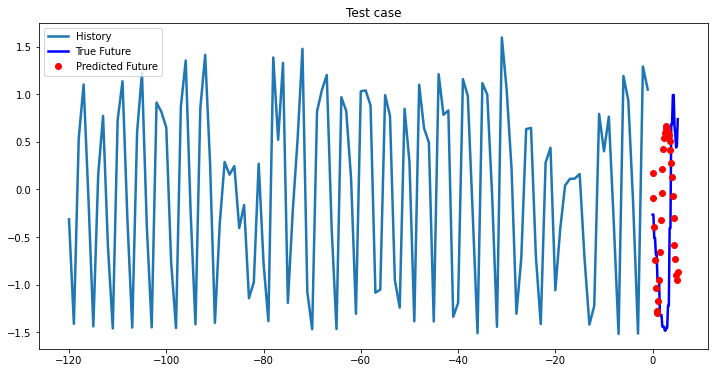
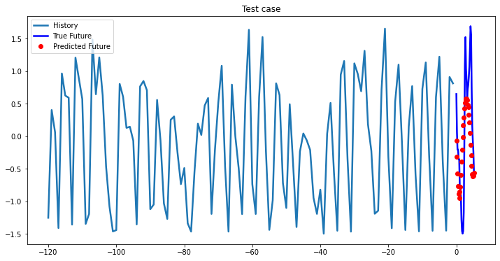
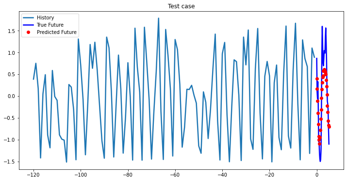
i = 0
while i < len(testX):
    test_x = testX[i].unsqueeze(0)
    test_y = testY[i].unsqueeze(0)
    multi_step_plot[test_x.numpy(](0, :, target_index), test_y.detach().numpy()[0, :], lstm_model(test_x).detach().numpy()[0, :], 'Test case')
    i += 100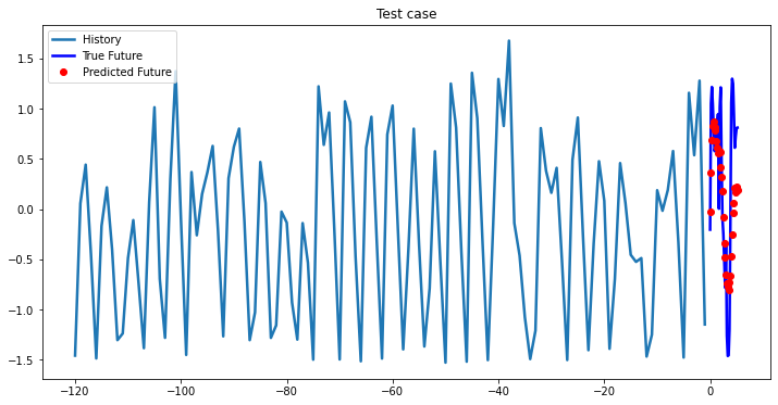

Out [33]:

2-Layer LSTM

In [34]:

learning_rate = 0.001
input_size = trainX.shape[2] # number of input features, multivariate case
hidden_size = 20
num_layers = 2
num_classes = trainY.shape[1] # future time window length
lstm_model = LSTMTimeSeriesPredictor(num_classes, input_size, hidden_size, num_layers, bidirectional=False)

config = {'batch_size': 128, 'num_epochs': 10, 'checkpoints_dir': '/content/drive/My Drive/time series prediction/', 'model_filename': '2-layer-lstm-best_model.pth.tar'}

criterion = torch.nn.MSELoss()
optimizer = torch.optim.Adam(lstm_model.parameters(), lr=learning_rate)

train_history, val_history = [], []

best_model_wts = copy.deepcopy(lstm_model.state_dict())

best_loss = 10e10

if not os.path.exists(config['checkpoints_dir']):
    os.mkdir(config['checkpoints_dir'])

for epoch in range(config['num_epochs']):
    print("="*20 + str(epoch+1) + "="*20)
    _, train_loss = train_model(lstm_model, train_data, criterion, optimizer, config['batch_size'])
    train_history.append(train_loss)

    _, val_loss, best_model_wts = evaluate_model(lstm_model, val_data, criterion, optimizer, config['batch_size'])
    val_history.append(val_loss)

    if val_loss < best_loss:
        best_loss = val_loss
        print("Saving model for best loss")
        checkpoint = {
            'state_dict': best_model_wts
        }
        torch.save(checkpoint, config['checkpoints_dir'] + config['model_filename'])
        best_model_wts = copy.deepcopy(lstm_model.state_dict())

Out [34]:

====================1====================
Epoch: 1, train loss: 0.89874
Epoch: 1, val loss: 0.77490
Saving model for best loss
====================2====================
Epoch: 2, train loss: 0.77985
Epoch: 2, val loss: 0.73741
Saving model for best loss
====================3====================
Epoch: 3, train loss: 0.75368
Epoch: 3, val loss: 0.71219
Saving model for best loss
====================4====================
Epoch: 4, train loss: 0.73283
Epoch: 4, val loss: 0.69299
Saving model for best loss
====================5====================
Epoch: 5, train loss: 0.71830
Epoch: 5, val loss: 0.68409
Saving model for best loss
====================6====================
Epoch: 6, train loss: 0.70771
Epoch: 6, val loss: 0.67732
Saving model for best loss
====================7====================
Epoch: 7, train loss: 0.69788
Epoch: 7, val loss: 0.67322
Saving model for best loss
====================8====================
Epoch: 8, train loss: 0.69050
Epoch: 8, val loss: 0.67194
Saving model for best loss
====================9====================
Epoch: 9, train loss: 0.68391
Epoch: 9, val loss: 0.66734
Saving model for best loss
====================10====================
Epoch: 10, train loss: 0.67748
Epoch: 10, val loss: 0.66578
Saving model for best loss

In [35]:

plt.plot(np.arange(config['num_epochs']), train_history, label='Train loss')
plt.plot(np.arange(config['num_epochs']), val_history, label='Val loss')
plt.xlabel("num of epochs")
plt.ylabel("train loss")
plt.show()

Out [35]:

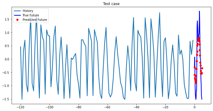
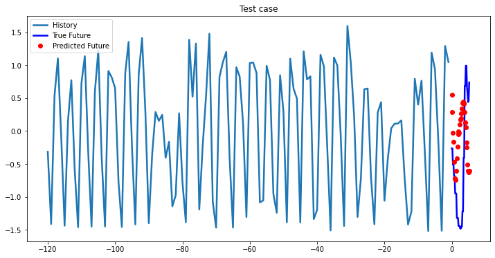
Test

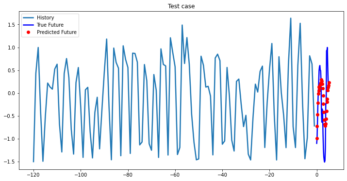
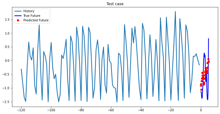
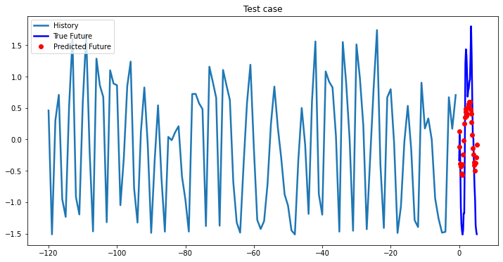
In [36]:

lstm_model = LSTMTimeSeriesPredictor(num_classes, input_size, hidden_size, num_layers)
lstm_model.load_state_dict(torch.load(os.path.join(config['checkpoints_dir'], config['model_filename']))['state_dict'])
lstm_model.eval()
for param in lstm_model.parameters():
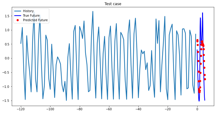
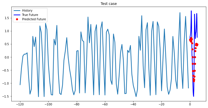
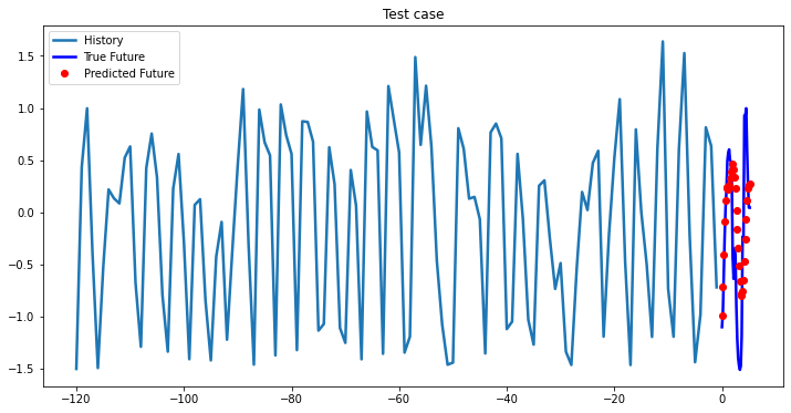
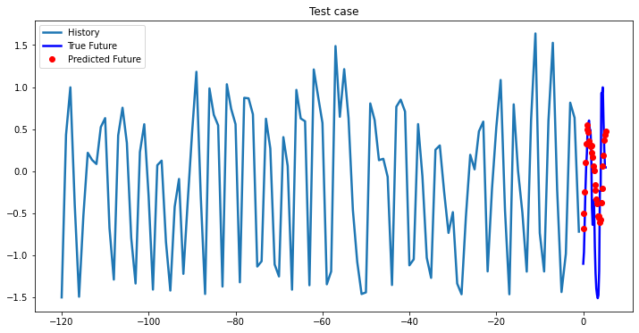
    param.requires_grad = False

In [37]:

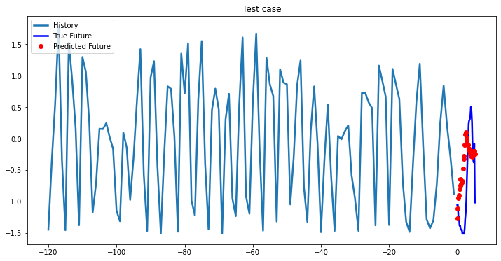
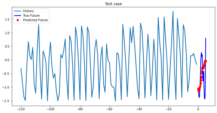
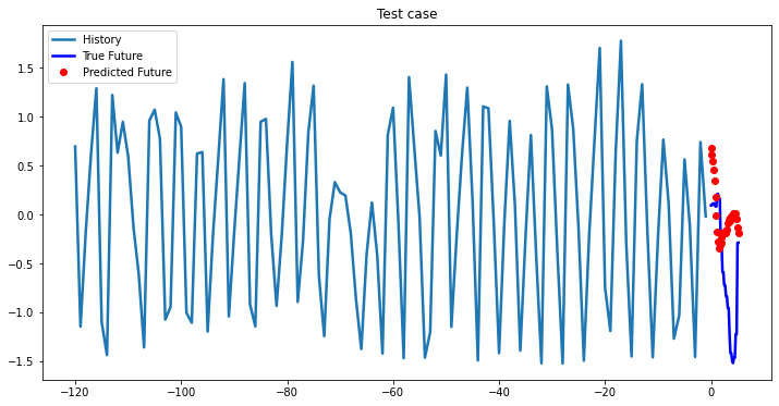
i = 0
while i < len(testX):
    test_x = testX[i].unsqueeze(0)
    test_y = testY[i].unsqueeze(0)
    multi_step_plot[test_x.numpy(](0, :, target_index), test_y.detach().numpy()[0, :], lstm_model(test_x).detach().numpy()[0, :], 'Test case')
    i += 100

Out [37]:

Bidirectional 1-Layer LSTM

In [38]:

learning_rate = 0.001
input_size = trainX.shape[2] # number of input features, multivariate case
hidden_size = 20
num_layers = 1
num_classes = trainY.shape[1] # future time window length
lstm_model = LSTMTimeSeriesPredictor(num_classes, input_size, hidden_size, num_layers, bidirectional=True)

config = {'batch_size': 128, 'num_epochs': 10, 'checkpoints_dir': '/content/drive/My Drive/time series prediction/', 'model_filename': 'bidir-1-layer-lstm-best_model.pth.tar'}

criterion = torch.nn.MSELoss()
optimizer = torch.optim.Adam(lstm_model.parameters(), lr=learning_rate)

train_history, val_history = [], []

best_model_wts = copy.deepcopy(lstm_model.state_dict())

best_loss = 10e10  # for validation phase

if not os.path.exists(config['checkpoints_dir']):
    os.mkdir(config['checkpoints_dir'])

for epoch in range(config['num_epochs']):
    print("="*20 + str(epoch+1) + "="*20)
    _, train_loss = train_model(lstm_model, train_data, criterion, optimizer, config['batch_size'])
    train_history.append(train_loss)

    _, val_loss, best_model_wts = evaluate_model(lstm_model, val_data, criterion, optimizer, config['batch_size'])
    val_history.append(val_loss)

    if val_loss < best_loss:
        best_loss = val_loss
        print("Saving model for best loss")
        checkpoint = {
            'state_dict': best_model_wts
        }
        torch.save(checkpoint, config['checkpoints_dir'] + config['model_filename'])
        best_model_wts = copy.deepcopy(lstm_model.state_dict())

Out [38]:

====================1====================
Epoch: 1, train loss: 0.92054
Epoch: 1, val loss: 0.78858
Saving model for best loss
====================2====================
Epoch: 2, train loss: 0.77843
Epoch: 2, val loss: 0.73070
Saving model for best loss
====================3====================
Epoch: 3, train loss: 0.75058
Epoch: 3, val loss: 0.71063
Saving model for best loss
====================4====================
Epoch: 4, train loss: 0.73297
Epoch: 4, val loss: 0.69804
Saving model for best loss
====================5====================
Epoch: 5, train loss: 0.71834
Epoch: 5, val loss: 0.68801
Saving model for best loss
====================6====================
Epoch: 6, train loss: 0.70628
Epoch: 6, val loss: 0.67993
Saving model for best loss
====================7====================
Epoch: 7, train loss: 0.69642
Epoch: 7, val loss: 0.67463
Saving model for best loss
====================8====================
Epoch: 8, train loss: 0.68780
Epoch: 8, val loss: 0.67683
====================9====================
Epoch: 9, train loss: 0.68003
Epoch: 9, val loss: 0.67213
Saving model for best loss
====================10====================
Epoch: 10, train loss: 0.67364
Epoch: 10, val loss: 0.66894
Saving model for best loss

In [39]:

plt.plot(np.arange(config['num_epochs']), train_history, label='Train loss')
plt.plot(np.arange(config['num_epochs']), val_history, label='Val loss')
plt.xlabel("num of epochs")
plt.ylabel("train loss")
plt.show()

Out [39]:

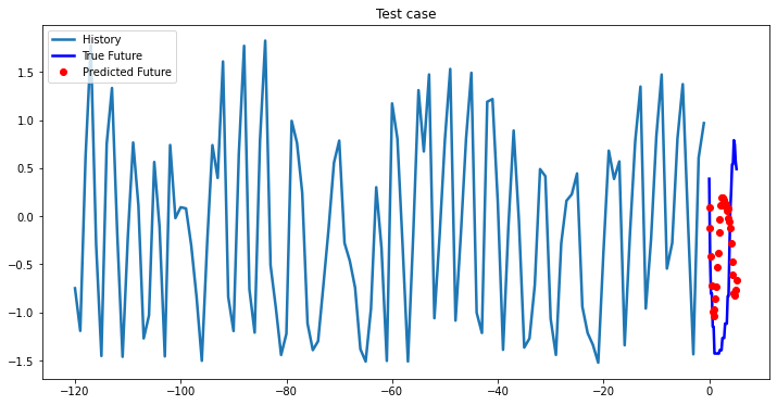
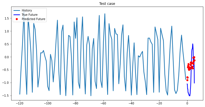
Test

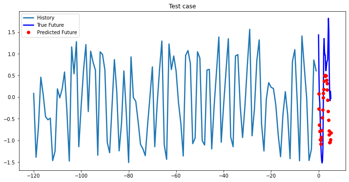
In [40]:

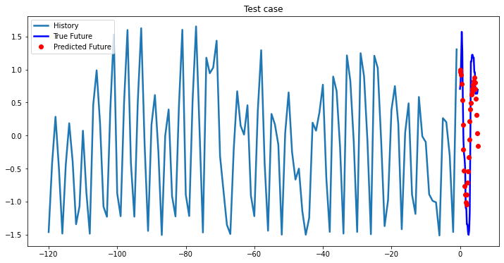
from collections import OrderedDict

state_dict = torch.load(os.path.join(config['checkpoints_dir'], config['model_filename']))['state_dict']

new_state_dict = OrderedDict()
for k,v in state_dict.items():
    if k not in ["lstm.weight_ih_l0_reverse", "lstm.weight_hh_l0_reverse", "lstm.bias_ih_l0_reverse", "lstm.bias_hh_l0_reverse"]:
        new_state_dict[k] = v

In [41]:

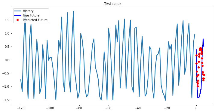
lstm_model = LSTMTimeSeriesPredictor(num_classes, input_size, hidden_size, num_layers)
lstm_model.load_state_dict(new_state_dict)
lstm_model.eval()
for param in lstm_model.parameters():
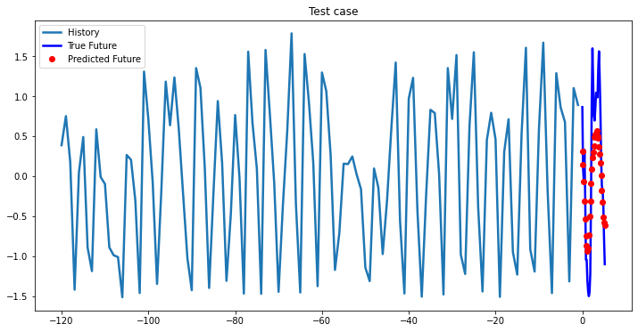
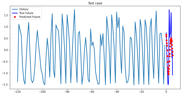
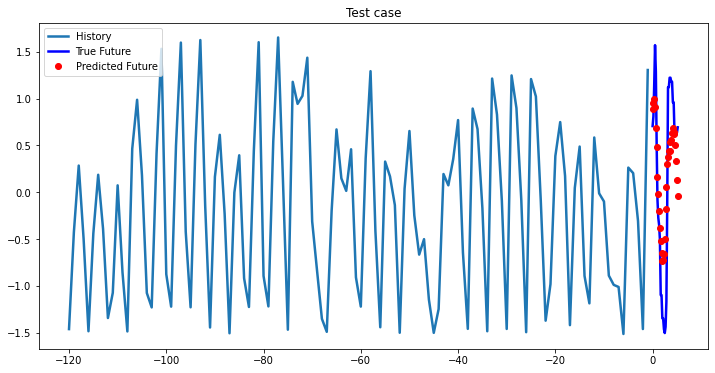
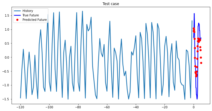
    param.requires_grad = False

In [42]:

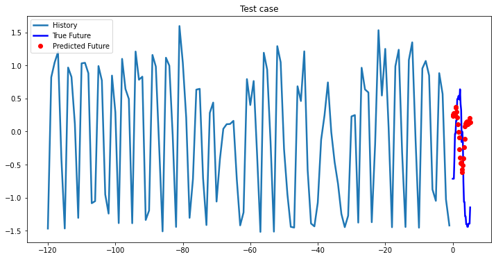
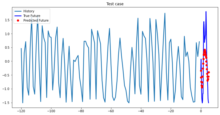
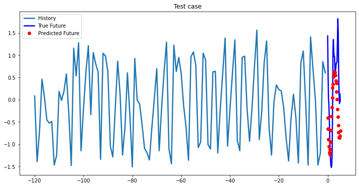
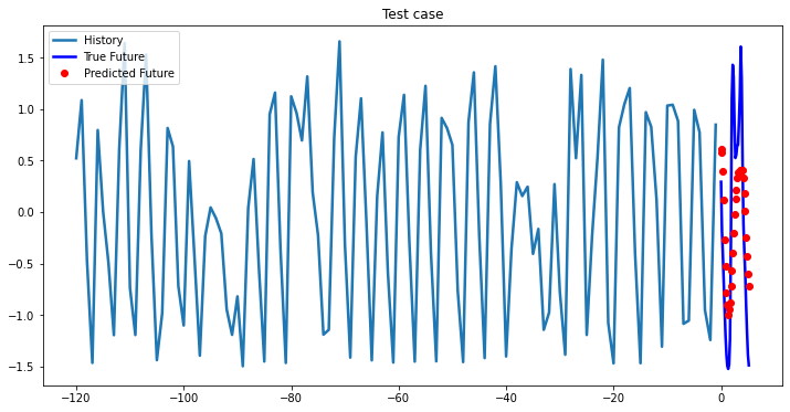
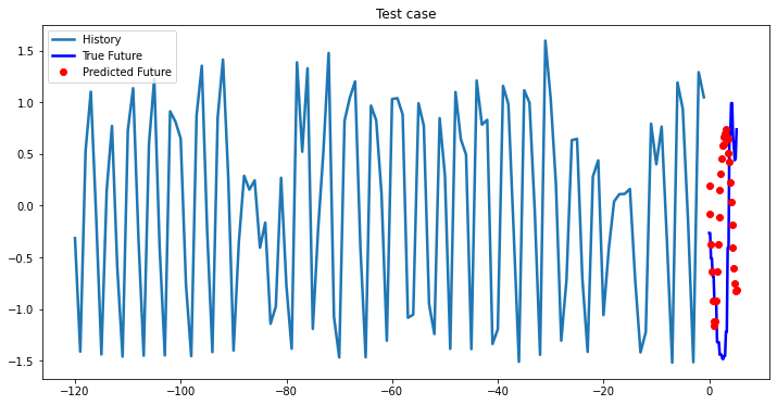
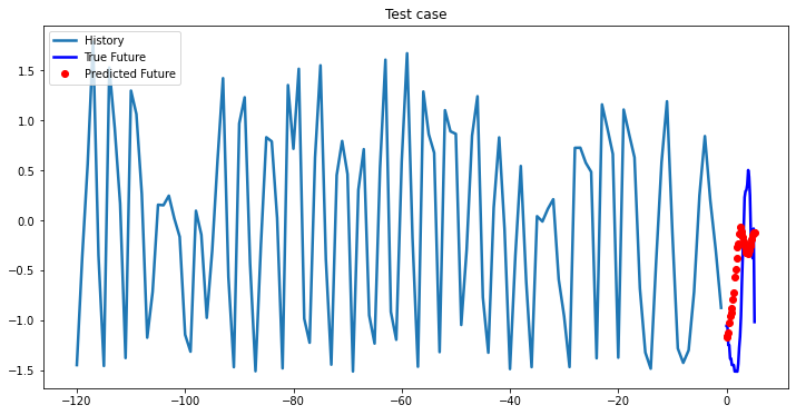
i = 0
while i < len(testX):
    test_x = testX[i].unsqueeze(0)
    test_y = testY[i].unsqueeze(0)
    multi_step_plot[test_x.numpy(](0, :, target_index), test_y.detach().numpy()[0, :], lstm_model(test_x).detach().numpy()[0, :], 'Test case')
    i += 100

Out [42]:

Experimental results on val data

Model	Best MSE loss
1-layer LSTM	0.66802
2-layer LSTM	0.66578
Bidirectional 1-layer LSTM	0.66894

Summary

At the first glance, all three models based on LSTM showed approximately the same results, so you can choose a single-layer LSTM without loss of quality. In cases where computational efficiency is a crucial part you may chose GRU model, which has less parameters to optimize than LSTM model. The ways you can improve existing deep learning model:

• work on data cleanliness, look for essential features, which are strongly related to the target variable;
• manual and automatic feature engineering;
• optimization of hyperparameters (length of hidden state vector, batch size, number of epochs, learning rate, number of layers);
• try different optimization algorithm;
• try different loss function which will be differentiable and adequate to task you’re solving;
• use ensembles of prediction vectors.