Graph Neural Networks for Fraud Detection in Crypto Transactions

In this tutorial, we apply Graph Convolutional Network (GCN) and Graph Attention Network (GAT) to detect fraudulent bitcoin transactions on the Elliptic dataset, and compare their performances.

Introduction

Despite significant progress within deep learning areas such as computer vision, natural language/audio processing, time series forecasting, etc., the majority of problems work with non-euclidian geometric data and as an example of such data are social network connections, IoT sensors topology, molecules, gene expression data and so on. The non-Euclidian nature of data implies that all properties of Euclidian vector space $\mathbf{R^n}$ can not be applied to such data samples; for example, shift-invariance, which is an important property for Convolutional Neural Networks (CNN), does not save her. In [1] the authors explain how convolution operation can be translated to the non-Euclidian domain using spectral convolution representation for graph structures. At present, Graph Neural Networks (GNN) have found their application in many areas:

• physics (particle systems simulation, robotics, object trajectory prediction)
• chemistry and biology (drug and protein interaction, protein interface prediction, cancer subtype detection, molecular fingerprints, chemical reaction prediction)
• combinatorial optimizations (used to solve NP-hard problems such as traveling salesman problem, minimum spanning trees)
• traffic networks (traffic prediction, taxi demand problem)
• recommendation systems (links prediction between users and content items, social network recommendations)
• computer vision (scene graph generation, point clouds classification, action recognition, semantic segmentation, few-shot image classification, visual reasoning)
• natural language processing (text classification, sequence labeling, neural machine translation, relation extraction, question answering) Among the classes of state-of-the-art GNNs, we can distinguish them into recurrent GNNs, convolutional GNNs, graph autoencoders, generative GNNs, and spatial-temporal GNNs.

In this tutorial, we will consider the semi-supervised node classification problems using Graph Convolutional Network and Graph Attention Network and compare their performances on the Elliptic dataset, which contains crypto transaction data. Also, we will highlight their building block concepts, which come from spectral-based and spatial-based representations of convolution.

Spectral-based GNN: Graph Convolutional Network (GCN)

Spectral-based models take their mathematical basis from the graph signal processing field; among known models are ChebNet, GCN, AGCN, and DGCN. To understand the principle of such models, let’s consider the concept of spectral convolution [2, 3].

Let’s say we have a graph signal $\mathbf{x}$ from $\mathbf{R^n}$, which is the feature vector of all nodes of a graph, and $\mathbf{x_i}$ is a value of a i-th node. This graph signal is first transformed to the spectral domain by applying Fourier transform to conduct a convolution operator. After the convolution, the resulting signal is transformed back using the inverse graph Fourier transform. These transforms are defined as:

$$\begin{aligned} \mathcal{F}(x) &= U^{T} x \\ \mathcal{F}^{-1}(x) &= Ux \end{aligned}$$

Here $\mathbf{U}$ is the matrix of eigenvectors of the normalized graph Laplacian

$$\begin{aligned} \mathbf{L} = \mathbf{I}_N - \mathbf{D}^{-1/2}\mathbf{A}\mathbf{D}^{-1/2} \end{aligned}$$

where $\mathbf{D}$ is the degree matrix, $\mathbf{A}$ is the adjacency matrix of the graph, and $\mathbf{I_{N}}$ is the identity matrix. The normalized graph Laplacian can be factorized as

$$\begin{aligned} L = U \Lambda U^{T} \end{aligned}$$

Based on the convolution theorem, the convolution operation with filter $\mathbf{g}$ can be defined as:

$$\begin{aligned} g \star x &= \mathcal{F}^{-1}\big(\mathcal{F}(g) \odot \mathcal{F}(x)\big) \\ &= U \left( U^{T} g \odot U^{T} x \right) \end{aligned}$$

if we denote a filter as $\mathbf{g}$ as a learnable diagonal matrix of $\mathbf{U^{T}g}$, then we get

$$\begin{aligned} g_{w} \star x = U \, g_{w} \, U^{T} x \end{aligned}$$

We can understand $\mathbf{g_{w}}$ as a function of the eigenvalues of $\mathbf{L}$. Evaluation of multiplication with the eigenvector matrix $\mathbf{U}$ takes O(N²) time complexity; to overcome this problem, in ChebNet and GCN, Chebyshev polynomials are used. For ChebNet, spectral convolution operation is represented as follows.

$$\begin{aligned} g_{w} \star x \approx \sum_{k=0}^{K} w_k \, T_k(\tilde{L}) \, x \end{aligned}$$ $$\begin{aligned} \tilde{L} = \frac{2}{\lambda_{\max}} L - I_{N} \end{aligned}$$

To circumvent the problem of overfitting, in GCN, Chebyshev approximation with $K=1$ and $\mathbf{\lambda_{max}}$ is used. And convolutional operator will become as follows.

$$\begin{aligned} g_{w} \star x &\approx w_0 x + w_1 (L - I_N) x \\ &= w_0 x - w_1 D^{-\frac{1}{2}} A D^{-\frac{1}{2}} x \end{aligned}$$

Assuming, $w = w_0 = - w_1$, we get

$$\begin{aligned} g_{w} \star x \approx w \left( I_N + D^{-\frac{1}{2}} A D^{-\frac{1}{2}} \right) x \end{aligned}$$

GCN further introduces a normalization trick to solve the exploding/vanishing gradient problem

$$\begin{aligned} I_N + D^{-\frac{1}{2}} A D^{-\frac{1}{2}} \;\rightarrow\; \tilde{D}^{-\frac{1}{2}} \tilde{A} \tilde{D}^{-\frac{1}{2}} \end{aligned}$$ $$\begin{aligned} \tilde{A} = A + I_N \end{aligned}$$ $$\begin{aligned} \tilde{D}_{ii} = \sum_{j} \tilde{A}_{ij} \end{aligned}$$

Finally, the compact form of GCN is defined as

$$\begin{aligned} H = \tilde{D}^{-\frac{1}{2}} \tilde{A} \tilde{D}^{-\frac{1}{2}} X W \end{aligned}$$

Here, $\mathbf{X}$ is the input feature matrix, $dim(\mathbf{X}) = {N} * F^0$, ${N}$ is the number of nodes, and $F^0$ number of input features for each node;

$\mathbf{A}$ is the adjacency matrix, $dim(\mathbf{A}) = {N} * {N}$;

$\mathbf{W}$ is the weights matrix, $dim(\mathbf{W}) = {F} * {F'}$, ${F}$ is the number of input features, ${F'}$ is the number of output features;

$\mathbf{H}$ represents a hidden layer of graph neural network, $dim(\mathbf{H}) = {N} * {F'}$.

At each i-th layer $H_i$, features are aggregated to form the next layer’s features, using the propagation rule $f$ (e.g. sigmoid/relu), and thus features become increasingly abstract at each consecutive layer, which reminds the principle of CNN.

Attention-based GNN: Graph Attention Network (GAT)

Among spatial-based convolutional GNN models, the following models are widely known: GraphSage, GAT, MoNet, GAAN, DiffPool, and others. The working principle is similar to CNN convolution operator application to image data, except the spatial approach applies convolution to differently sized node neighbors of a graph.

Attention mechanism gained wide popularity thanks to the models used in NLP tasks (e.g., LSTM with attention, transformers). In the case of GNN having an attention mechanism, contributions of neighboring nodes to the considered node are neither identical nor pre-defined, as, for example, in GraphSage or GCN models.

Let’s look at the attention mechanism of GAT [4]; normalized attention coefficients for this model can be calculated via the following formula:

$$\begin{aligned} \alpha_{ij} = \frac{ \exp\left( \text{LeakyReLU}\left( \vec{a}^{\,T} \left[ W \vec{h}_i \,\|\, W \vec{h}_j \right] \right) \right) }{ \sum_{k \in \mathcal{N}_i} \exp\left( \text{LeakyReLU}\left( \vec{a}^{\,T} \left[ W \vec{h}_i \,\|\, W \vec{h}_k \right] \right) \right) } \end{aligned}$$

Here, $T$ represents transposition and $\|$ is concatenation operation;

$\mathbf{h}$ is a set of node features ($N$ is a number of nodes, $F$ is a number of features in each node)

$$\begin{aligned} \mathbf{h} = \{ \vec{h}_1, \vec{h}_2, \ldots, \vec{h}_N \}, \quad \vec{h}_i \in \mathbb{R}^F \end{aligned}$$

$\mathbf{w}$ is weight matrix (linear transformation to a features), $dim(\mathbf{W}) = {F'} * {F}$.

Vector $\mathbf{a}$ is the weight vector for a single-layer feed-forward neural network

$$\begin{aligned} \vec{a} \in \mathbb{R}^{2F'} \end{aligned}$$

The softmax function ensures that the attention weights sum up to one overall neighbour of the i-th node.

Finally, these normalized attention coefficients are used to compute a linear combination of the features corresponding to them, to serve as the final output features for every node.

$$\begin{aligned} \vec{h}_i^{\,\prime} = \sigma \left( \sum_{j \in \mathcal{N}_i} \alpha_{ij} \, W \vec{h}_j \right) \end{aligned}$$

Usage of single self-attention can lead to instabilities, and in this case, multi-head attention with K independent attention mechanisms is used

$$\begin{aligned} \vec{h}_i^{\,\prime} = \big\Vert_{k=1}^{K} \sigma \left( \sum_{j \in \mathcal{N}_i} \alpha_{ij}^{k} \, W^{k} \vec{h}_j \right) \end{aligned}$$

Dataset: Elliptic Bitcoin

Here, for the node classification task, we will use the Elliptic dataset contains:

• 203,769 nodes (Bitcoin transactions)
• 234,355 edges (transaction flows)
• 3 node classes: licit, illicit, unknown

Node classification with GCN/GAT using PyTorch Geometric (PyG)

Here we will consider a semi-supervised node classification problem using PyG library, where nodes will be transactions and edges will be transactions flows.

import os
import copy
import torch
import warnings
import numpy as np
import pandas as pd
import networkx as nx
import seaborn as sns
import matplotlib.pyplot as plt

from sklearn.metrics import confusion_matrix, classification_report
from sklearn.model_selection import train_test_split

from torch_geometric.utils import to_networkx
from torch_geometric.data import Data, DataLoader

import torch.nn.functional as F
from torch.nn import Linear, Dropout
from torch_geometric.nn import GCNConv, GATv2Conv

warnings.filterwarnings('ignore')

You can simply import the Elliptic bitcoin dataset from PyG pre-installed datasets using the instructions down below, but for the sake of clarity, let’s build PyG dataset object by ourselves. Raw data can be downloaded via this link.

from torch_geometric.datasets import EllipticBitcoinDataset
dataset = EllipticBitcoinDataset(root=’./data/elliptic-bitcoin-dataset’)

class Config:
    seed = 0
    learning_rate = 0.001
    weight_decay = 1e-5
    input_dim = 165
    output_dim = 1
    hidden_size = 128
    num_epochs = 100
    checkpoints_dir = './models/elliptic_gnn'
    device = torch.device('cuda' if torch.cuda.is_available() else 'cpu')

print("Using device:", Config.device)

Data loading/preparation

For the data preparation, I used this Kaggle notebook as a basis.

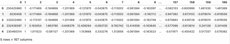
df_features = pd.read_csv('./data/elliptic_bitcoin_dataset/elliptic_txs_features.csv', header=None)
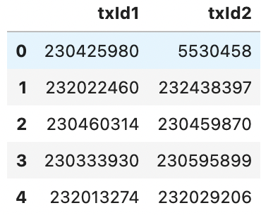
df_edges = pd.read_csv("./data/elliptic_bitcoin_dataset/elliptic_txs_edgelist.csv")
df_classes =  pd.read_csv("./data/elliptic_bitcoin_dataset/elliptic_txs_classes.csv")
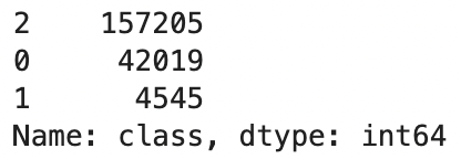
df_classes['class'] = df_classes['class'].map({'unknown': 2, '1': 1, '2': 0})

# here column 0 stands for node_id, column 1 is the time axis
df_features.head()

df_edges.head()

0 — legitimate
1 — fraud
2 — unknown class

df_classes['class'].value_counts()

# merging node features DF with classes DF
df_merge = df_features.merge(df_classes, how='left', right_on="txId", left_on=0)
df_merge = df_merge.sort_values(0).reset_index(drop=True)

# extracting classified/non-classified nodes
classified = df_merge.loc[df_merge['class'].loc[df_merge['class']!=2].index].drop('txId', axis=1)
unclassified = df_merge.loc[df_merge['class'].loc[df_merge['class']==2].index].drop('txId', axis=1)

# extracting classified/non-classified edges
classified_edges = df_edges.loc[df_edges['txId1'].isin(classified[0]) & df_edges['txId2'].isin(classified[0])]
unclassifed_edges = df_edges.loc[df_edges['txId1'].isin(unclassified[0]) | df_edges['txId2'].isin(unclassified[0])]

Preparing edges

# mapping nodes to indices
nodes = df_merge[0].values
map_id = {j:i for i,j in enumerate(nodes)}

# mapping edges to indices
edges = df_edges.copy()
edges.txId1 = edges.txId1.map(map_id)
edges.txId2 = edges.txId2.map(map_id)
edges = edges.astype(int)

edge_index = np.array(edges.values).T
edge_index = torch.tensor(edge_index, dtype=torch.long).contiguous()

# weights for the edges are equal in case of model without attention
weights = torch.tensor([1] * edge_index.shape[1] , dtype=torch.float32)

print("Total amount of edges in DAG:", edge_index.shape)

Total amount of edges in DAG: torch.Size([2, 234355])

Preparing nodes

Let’s ignore the temporal axis and consider the static case of fraud detection.

# maping node ids to corresponding indexes
node_features = df_merge.drop(['txId'], axis=1).copy()
node_features[0] = node_features[0].map(map_id)

classified_idx = node_features['class'].loc[node_features['class']!=2].index
unclassified_idx = node_features['class'].loc[node_features['class']==2].index

# replace unkown class with 0, to avoid having 3 classes, this data/labels never used in training
node_features['class'] = node_features['class'].replace(2, 0)

labels = node_features['class'].values

# drop indeces, class and temporal axes
node_features = torch.tensor(np.array(node_features.drop([0, 'class', 1], axis=1).values, dtype=np.float32), dtype=torch.float32)

PyG Dataset

# converting data to PyGeometric graph data format
elliptic_dataset = Data(x = node_features,
                        edge_index = edge_index,
                        edge_attr = weights,
                        y = torch.tensor(labels, dtype=torch.float32))

print(f'Number of nodes: {elliptic_dataset.num_nodes}')
print(f'Number of node features: {elliptic_dataset.num_features}')
print(f'Number of edges: {elliptic_dataset.num_edges}')
print(f'Number of edge features: {elliptic_dataset.num_features}')
print(f'Average node degree: {elliptic_dataset.num_edges / elliptic_dataset.num_nodes:.2f}')
print(f'Number of classes: {len(np.unique(elliptic_dataset.y))}')
print(f'Has isolated nodes: {elliptic_dataset.has_isolated_nodes()}')
print(f'Has self loops: {elliptic_dataset.has_self_loops()}')
print(f'Is directed: {elliptic_dataset.is_directed()}')

Number of nodes: 203769
Number of node features: 165
Number of edges: 234355
Number of edge features: 165
Average node degree: 1.15
Number of classes: 2
Has isolated nodes: False
Has self loops: False
Is directed: True

y_train = labels[classified_idx]

# spliting train set and validation set
_, _, _, _, train_idx, valid_idx = \
    train_test_split(node_features[classified_idx],
                     y_train,
                     classified_idx,
                     test_size=0.15,
                     random_state=Config.seed,
                     stratify=y_train)

elliptic_dataset.train_idx = torch.tensor(train_idx, dtype=torch.long)
elliptic_dataset.val_idx = torch.tensor(valid_idx, dtype=torch.long)
elliptic_dataset.test_idx = torch.tensor(unclassified_idx, dtype=torch.long)

print("Train dataset size:", elliptic_dataset.train_idx.shape[0])
print("Validation dataset size:", elliptic_dataset.val_idx.shape[0])
print("Test dataset size:", elliptic_dataset.test_idx.shape[0])

Train dataset size: 39579
Validation dataset size: 6985
Test dataset size: 157205

Models Definitions

class GCN(torch.nn.Module):
    """Graph Convolutional Network"""
    def __init__(self, dim_in, dim_h, dim_out):
        super(GCN, self).__init__()

        self.gcn1 = GCNConv(dim_in, dim_h)
        self.gcn2 = GCNConv(dim_h, dim_out)

    def forward(self, x, edge_index):
        h = self.gcn1(x, edge_index)
        h = torch.relu(h)
        h = F.dropout(h, p=0.6, training=self.training)
        out = self.gcn2(h, edge_index)
        return out

class GAT(torch.nn.Module):
    """Graph Attention Network"""
    def __init__(self, dim_in, dim_h, dim_out, heads=8):
        super(GAT, self).__init__()
        self.gat1 = GATv2Conv(dim_in, dim_h, heads=heads, dropout=0.6)
        self.gat2 = GATv2Conv(dim_h*heads, dim_out, concat=False, heads=1, dropout=0.6)

    def forward(self, x, edge_index):
        h = F.dropout(x, p=0.6, training=self.training)
        h = self.gat1(h, edge_index)
        h = F.elu(h)
        h = F.dropout(h, p=0.6, training=self.training)
        out = self.gat2(h, edge_index)
        return out

def accuracy(y_pred, y_test, prediction_threshold=0.5):
    y_pred_label = (torch.sigmoid(y_pred) > prediction_threshold).float()*1

    correct_results_sum = (y_pred_label == y_test).sum().float()
    acc = correct_results_sum/y_test.shape[0]

    return acc

Training Loop

def train_evaluate(model, data, criterion, optimizer, *args):
    num_epochs = args[0]
    checkpoints_dir = args[1]
    model_filename = args[2]

    best_model_wts = copy.deepcopy(model.state_dict())

    best_loss = 10e10

    if not os.path.exists(checkpoints_dir):
        os.makedirs(checkpoints_dir)

    model.train()
    for epoch in range(num_epochs+1):
        # Training
        optimizer.zero_grad()
        out = model(data.x, data.edge_index)
        loss = criterion(out[data.train_idx], data.y[data.train_idx].unsqueeze(1))
        acc = accuracy(out[data.train_idx], data.y[data.train_idx].unsqueeze(1), prediction_threshold=0.5)
        loss.backward()
        optimizer.step()

        # Validation
        val_loss = criterion(out[data.val_idx], data.y[data.val_idx].unsqueeze(1))
        val_acc = accuracy(out[data.val_idx], data.y[data.val_idx].unsqueeze(1), prediction_threshold=0.5)

        if(epoch % 10 == 0):
            print(f'Epoch {epoch:>3} | Train Loss: {loss:.3f} | Train Acc: '
                  f'{acc*100:>6.2f}% | Val Loss: {val_loss:.2f} | '
                  f'Val Acc: {val_acc*100:.2f}%')

            if val_loss < best_loss:
                best_loss = val_loss
                print("Saving model for best loss")
                checkpoint = {
                    'state_dict': best_model_wts
                }
                torch.save(checkpoint, os.path.join(checkpoints_dir, model_filename))
                best_model_wts = copy.deepcopy(model.state_dict())

    return model

def test(model, data):
    model.eval()
    out = model(data.x, data.edge_index)
    preds = ((torch.sigmoid(out) > 0.5).float()*1).squeeze(1)
    return preds

Train GCN

gcn_model = GCN(Config.input_dim, Config.hidden_size, Config.output_dim).to(Config.device)
data_train = elliptic_dataset.to(Config.device)

optimizer = torch.optim.Adam(gcn_model.parameters(), lr=Config.learning_rate, weight_decay=Config.weight_decay)
scheduler = torch.optim.lr_scheduler.ReduceLROnPlateau(optimizer, 'min')
criterion = torch.nn.BCEWithLogitsLoss()

train_evaluate(gcn_model,
              data_train,
              criterion,
              optimizer,
              Config.num_epochs,
              Config.checkpoints_dir,
              'gcn_best_model.pth.tar')

Epoch 0 | Train Loss: 0.759 | Train Acc: 62.16% | Val Loss: 0.73 | Val Acc: 64.07%
Saving model for best loss
Epoch 10 | Train Loss: 0.307 | Train Acc: 86.43% | Val Loss: 0.30 | Val Acc: 87.16%
Saving model for best loss
Epoch 20 | Train Loss: 0.258 | Train Acc: 89.52% | Val Loss: 0.25 | Val Acc: 89.61%
Saving model for best loss
Epoch 30 | Train Loss: 0.244 | Train Acc: 90.49% | Val Loss: 0.24 | Val Acc: 90.32%
Saving model for best loss
Epoch 40 | Train Loss: 0.230 | Train Acc: 91.32% | Val Loss: 0.22 | Val Acc: 91.40%
Saving model for best loss
Epoch 50 | Train Loss: 0.219 | Train Acc: 91.85% | Val Loss: 0.22 | Val Acc: 91.77%
Saving model for best loss
Epoch 60 | Train Loss: 0.214 | Train Acc: 92.35% | Val Loss: 0.21 | Val Acc: 92.61%
Saving model for best loss
Epoch 70 | Train Loss: 0.210 | Train Acc: 92.60% | Val Loss: 0.21 | Val Acc: 92.80%
Saving model for best loss
Epoch 80 | Train Loss: 0.201 | Train Acc: 92.86% | Val Loss: 0.20 | Val Acc: 92.81%
Saving model for best loss
Epoch 90 | Train Loss: 0.195 | Train Acc: 93.15% | Val Loss: 0.20 | Val Acc: 92.81%
Saving model for best loss
Epoch 100 | Train Loss: 0.194 | Train Acc: 93.25% | Val Loss: 0.19 | Val Acc: 93.53%
Saving model for best loss

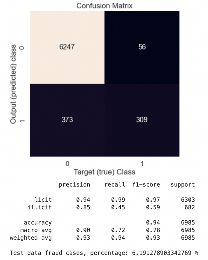
Test GCN

gcn_model.load_state_dict(torch.load(os.path.join(Config.checkpoints_dir, 'gcn_best_model.pth.tar'))['state_dict'])

y_test_preds = test(gcn_model, data_train)

# confusion matrix on validation data
conf_mat = confusion_matrix(data_train.y[data_train.val_idx].detach().cpu().numpy(), y_test_preds[valid_idx])

plt.subplots(figsize=(6,6))
sns.set(font_scale=1.4)
sns.heatmap(conf_mat, annot=True, fmt=".0f", annot_kws={"size": 16}, cbar=False)
plt.xlabel('Target (true) Class'); plt.ylabel('Output (predicted) class'); plt.title('Confusion Matrix')
plt.show();

print(classification_report(data_train.y[data_train.val_idx].detach().cpu().numpy(),
                            y_test_preds[valid_idx],
                            target_names=['licit', 'illicit']))


print(f"Test data fraud cases, percentage: {y_test_preds[data_train.test_idx].detach().cpu().numpy().sum() / len(data_train.y[data_train.test_idx]) *100} %")

Train GAT

gat_model = GAT(Config.input_dim, Config.hidden_size, Config.output_dim).to(Config.device)
data_train = elliptic_dataset.to(Config.device)

optimizer = torch.optim.Adam(gat_model.parameters(), lr=Config.learning_rate, weight_decay=Config.weight_decay)
scheduler = torch.optim.lr_scheduler.ReduceLROnPlateau(optimizer, 'min')
criterion = torch.nn.BCEWithLogitsLoss()

train_evaluate(gat_model,
               data_train,
               criterion,
               optimizer,
               Config.num_epochs,
               Config.checkpoints_dir,
               'gat_best_model.pth.tar')

Epoch 0 | Train Loss: 1.176 | Train Acc: 68.34% | Val Loss: 1.01 | Val Acc: 68.33%
Saving model for best loss
Epoch 10 | Train Loss: 0.509 | Train Acc: 88.63% | Val Loss: 0.48 | Val Acc: 88.70%
Saving model for best loss
Epoch 20 | Train Loss: 0.489 | Train Acc: 90.09% | Val Loss: 0.49 | Val Acc: 89.94%
Epoch 30 | Train Loss: 0.465 | Train Acc: 89.87% | Val Loss: 0.48 | Val Acc: 89.76%
Saving model for best loss
Epoch 40 | Train Loss: 0.448 | Train Acc: 89.81% | Val Loss: 0.44 | Val Acc: 90.15%
Saving model for best loss
Epoch 50 | Train Loss: 0.445 | Train Acc: 90.04% | Val Loss: 0.44 | Val Acc: 89.89%
Epoch 60 | Train Loss: 0.443 | Train Acc: 90.22% | Val Loss: 0.44 | Val Acc: 90.45%
Epoch 70 | Train Loss: 0.439 | Train Acc: 90.38% | Val Loss: 0.43 | Val Acc: 90.16%
Saving model for best loss
Epoch 80 | Train Loss: 0.426 | Train Acc: 90.57% | Val Loss: 0.43 | Val Acc: 90.41%
Saving model for best loss
Epoch 90 | Train Loss: 0.423 | Train Acc: 90.72% | Val Loss: 0.42 | Val Acc: 90.38%
Saving model for best loss
Epoch 100 | Train Loss: 0.418 | Train Acc: 90.72% | Val Loss: 0.42 | Val Acc: 90.74%
Saving model for best loss

Test GAT

gat_model.load_state_dict(torch.load(os.path.join(Config.checkpoints_dir, 'gat_best_model.pth.tar'))['state_dict'])

y_test_preds = test(gat_model, data_train)

# confusion matrix on validation data
conf_mat = confusion_matrix(data_train.y[data_train.val_idx].detach().cpu().numpy(), y_test_preds[valid_idx])

plt.subplots(figsize=(6,6))
sns.set(font_scale=1.4)
sns.heatmap(conf_mat, annot=True, fmt=".0f", annot_kws={"size": 16}, cbar=False)
plt.xlabel('Target (true) Class'); plt.ylabel('Output (predicted) class'); plt.title('Confusion Matrix')
plt.show();

print(classification_report(data_train.y[data_train.val_idx].detach().cpu().numpy(),
                            y_test_preds[valid_idx],
                            target_names=['licit', 'illicit']))


print(f"Test data fraud cases, percentage: {y_test_preds[data_train.test_idx].detach().cpu().numpy().sum() / len(data_train.y[data_train.test_idx]) *100} %")

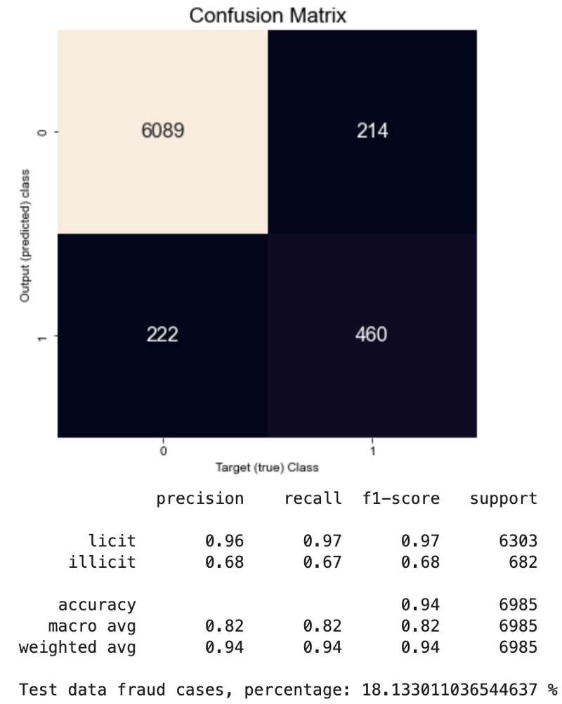
Results Comparison

Model	Val Accuracy	Illicit Recall	Test Fraud %
GCN	93.5%	0.45	~6%
GAT	90.7%	0.67	~18%

Key finding: GAT converges slower and has slightly lower overall accuracy, but the confusion matrix on labeled validation data shows recall for the illicit class improved from 0.45 → 0.67. GAT more correctly identifies fraudsters, at the cost of being stricter on licit transactions.

The test set (157,205 unlabeled samples) contains ~6% fraud predictions from GCN versus ~18% from GAT — suggesting GAT may be recovering many true positives that GCN misses.

Full code: GitHub

References

1. Bronstein et al., Geometric deep learning: going beyond Euclidean data (2017)
2. Kipf & Welling, Semi-supervised classification with graph convolutional networks (2017)
3. Zhou et al., Graph neural networks: A review of methods and applications (2020)
4. Veličković et al., Graph Attention Networks (2018)