In this tutorial we will consider colorectal histology tissues classification using ResNet architecture and PyTorch framework.
Introduction
Recently machine learning (ML) applications became widespread in the healthcare industry: omics field (genomics, transcriptomics, proteomics), drug investigation, radiology and digital histology. Deep learning based image analysis studies in histopathology include different tasks (e.g., classification, semantic segmentation, detection, and instance segmentation). The main goal of ML in this field is automatic detection, grading and prognosis of cancer.
However, there are several challenges in digital pathology. Usually histology slides are large sized hematoxylin and eosin (H&E) stained images with color variations and artifacts; different levels of magnification result in different levels of information extraction. One Whole Slide Image (WSI) is a multi-gigabyte image with typical resolution 100,000 × 100,000 pixels.
In a supervised classification scenario, WSIs are divided into patches with some stride, then a CNN architecture extracts feature vectors from patches which can be passed into traditional ML algorithms (SVM, gradient boosting) for further operations.
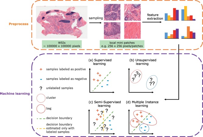
In this article we apply CNN ResNet architecture to classify tissue types of colon. We won't use transfer learning — weights from ImageNet are not related to histology and won't help convergence.
Dataset
The collection of textures in colorectal cancer histology — a "MNIST for biologists". Available at:
Two folders:
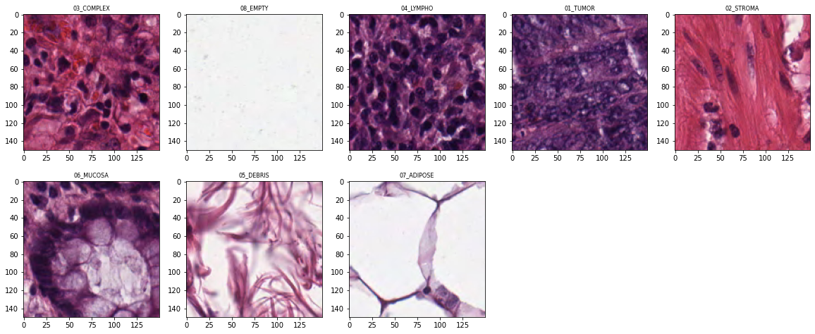
- 5000 image tiles: 150 × 150 px each (74 × 74 µm). Eight tissue categories.
- 10 larger images: 5000 × 5000 px each. Multiple tissue types per image.
All images are RGB, 0.495 µm/pixel, digitized with Aperio ScanScope, magnification 20×. Histological samples are fully anonymized images of formalin-fixed paraffin-embedded human colorectal adenocarcinomas from the University Medical Center Mannheim, Germany.
Colorectal MNIST Classification with ResNet
![]()
Setup
import os
import random
import itertools

import numpy as np
import pandas as pd
import matplotlib.pyplot as plt
from sklearn.model_selection import train_test_split
from PIL import Image
from sklearn.metrics import confusion_matrix, classification_report
import torch
import torch.nn as nn
import torch.utils.data as D
import torch.nn.functional as F
from torchvision import transforms, models
from tqdm import tqdm

import warnings
warnings.filterwarnings('ignore')

torch.cuda.empty_cache()DATA_DIR = '/kaggle/input/colorectal-histology-mnist/'
SMALL_IMG_DATA_DIR = os.path.join(DATA_DIR,
'kather_texture_2016_image_tiles_5000/Kather_texture_2016_image_tiles_5000')
IMAGE_SIZE = 224
SEED = 2000
BATCH_SIZE = 64
NUM_EPOCHS = 15
random.seed(SEED)
np.random.seed(SEED)
torch.manual_seed(SEED)
torch.cuda.manual_seed(SEED)
torch.backends.cudnn.deterministic = True
device = torch.device("cuda:0" if torch.cuda.is_available() else "cpu")Data Exploration
classes = os.listdir(SMALL_IMG_DATA_DIR)
classes['03_COMPLEX', '08_EMPTY', '04_LYMPHO', '01_TUMOR', '02_STROMA', '06_MUCOSA', '05_DEBRIS', '07_ADIPOSE']
for label in classes:
  num_samples = len(os.listdir(os.path.join(SMALL_IMG_DATA_DIR, label)))
print(label + ' ' + str(num_samples))03_COMPLEX 625 08_EMPTY 625 04_LYMPHO 625 01_TUMOR 625 02_STROMA 625 06_MUCOSA 625 05_DEBRIS 625 07_ADIPOSE 625
Sample tiles from each class:
PyTorch Dataset and DataLoaders
class HistologyMnistDS(D.Dataset):
  def __init__(self, df, transforms, mode='train'):
      self.records = df.to_records(index=False)
      self.transforms = transforms
      self.mode = mode
      self.len = df.shape[0]

  @staticmethod
  def _load_image_pil(path):
      return Image.open(path)

  def __getitem__(self, index):
      path = self.records[index].img_path
      img = self._load_image_pil(path)
      if self.transforms:
          img = self.transforms(img)
      if self.mode in ['train', 'val', 'test']:
          return img, torch.from_numpy(np.array(self.records[index].label_num))
      return img

  def __len__(self):
return self.lentrain_transforms = transforms.Compose([
transforms.Resize((IMAGE_SIZE, IMAGE_SIZE)),
transforms.ToTensor(),
transforms.Normalize([0.485, 0.456, 0.406], [0.229, 0.224, 0.225])
])
val_transforms = transforms.Compose([
transforms.Resize((IMAGE_SIZE, IMAGE_SIZE)),
transforms.ToTensor(),
transforms.Normalize([0.485, 0.456, 0.406], [0.229, 0.224, 0.225])
])train_df, tmp_df = train_test_split(df, test_size=0.2,
random_state=SEED, stratify=df['label'])
valid_df, test_df = train_test_split(tmp_df, test_size=0.8,
random_state=SEED, stratify=tmp_df['label'])
print("Train DF shape:", train_df.shape)
print("Valid DF shape:", valid_df.shape)
print("Test DF shape:", test_df.shape)Train DF shape: (4000, 3) Valid DF shape: (200, 3) Test DF shape: (800, 3)
ds_train = HistologyMnistDS(train_df, train_transforms)
ds_val = HistologyMnistDS(valid_df, val_transforms, mode='val')
ds_test = HistologyMnistDS(test_df, val_transforms, mode='test')
train_loader = D.DataLoader(ds_train, batch_size=BATCH_SIZE, shuffle=True, num_workers=4)
val_loader = D.DataLoader(ds_val, batch_size=BATCH_SIZE, shuffle=False, num_workers=4)
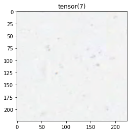
test_loader = D.DataLoader(ds_test, batch_size=BATCH_SIZE, shuffle=False, num_workers=4)Example batch image (denormalised):
Train Loop
import copy

checkpoints_dir = '/kaggle/working/'
history_train_loss, history_val_loss = [], []

def train_model(model, loss, optimizer, scheduler, num_epochs):
  best_model_wts = copy.deepcopy(model.state_dict())
  best_loss = 10e10
  best_acc_score = 0.0

  for epoch in range(num_epochs):
      print('Epoch {}/{}:'.format(epoch, num_epochs - 1), flush=True)

      for phase in ['train', 'val']:
          dataloader = train_loader if phase == 'train' else val_loader
          if phase == 'train':
              scheduler.step()
              model.train()
          else:
              model.eval()

          running_loss = running_acc = 0.

          for inputs, labels in tqdm(dataloader):
              inputs = inputs.to(device)
              labels = labels.to(device)
              optimizer.zero_grad()

              with torch.set_grad_enabled(phase == 'train'):
                  preds = model(inputs)
                  loss_value = loss(preds, labels)
                  preds_class = preds.argmax(dim=1)
                  if phase == 'train':
                      loss_value.backward()
                      optimizer.step()

              running_loss += loss_value.item()
              running_acc  += (preds_class == labels.data).float().mean()

          epoch_loss = running_loss / len(dataloader)
          epoch_acc  = running_acc  / len(dataloader)
          print(f'{phase} Loss: {epoch_loss:.4f}  Acc: {epoch_acc:.4f}', flush=True)

          if phase == 'train':
              history_train_loss.append(epoch_loss)
          else:
              history_val_loss.append(epoch_loss)
              if epoch_loss < best_loss:
                  best_loss = epoch_loss
                  best_model_wts = copy.deepcopy(model.state_dict())
                  print("Saving model for best loss")
                  os.makedirs(checkpoints_dir, exist_ok=True)
                  torch.save({'state_dict': best_model_wts},
                             checkpoints_dir + 'best_model.pth.tar')
              if epoch_acc > best_acc_score:
                  best_acc_score = epoch_acc
              print(f'Best loss: {best_loss:.4f}  Best acc: {best_acc_score:.4f}')

  return model
Model Setup and Training
ResNet-50 with the final linear layer replaced to output 8 classes. StepLR reduces the Adam learning rate by 10× every 7 epochs.
model = models.resnet50(pretrained=False)
model.fc = torch.nn.Linear(model.fc.in_features, len(classes))
model = model.to(device)

loss      = torch.nn.CrossEntropyLoss()
optimizer = torch.optim.Adam(model.parameters(), lr=1e-3)
scheduler = torch.optim.lr_scheduler.StepLR(optimizer, step_size=7, gamma=0.1)train_model(model, loss, optimizer, scheduler, num_epochs=NUM_EPOCHS);Epoch 0/14: val Loss: 0.7102 Acc: 0.7578 → Saving Epoch 2/14: val Loss: 0.4103 Acc: 0.8477 → Saving Epoch 6/14: val Loss: 0.1979 Acc: 0.9414 → Saving Epoch 9/14: val Loss: 0.1765 Acc: 0.9414 → Saving
Results
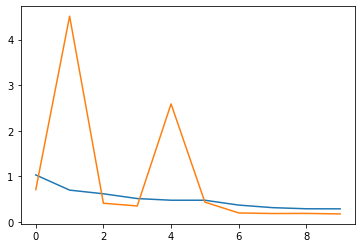
Train/validation loss curves:
model.load_state_dict(
  torch.load(os.path.join(checkpoints_dir, 'best_model.pth.tar'))['state_dict']
)
model.eval()

y_preds = []
for inputs, labels in tqdm(test_loader):
  inputs = inputs.to(device)
  with torch.set_grad_enabled(False):
      preds = model(inputs)
  y_preds.append(preds.argmax(dim=1).data.cpu().numpy())
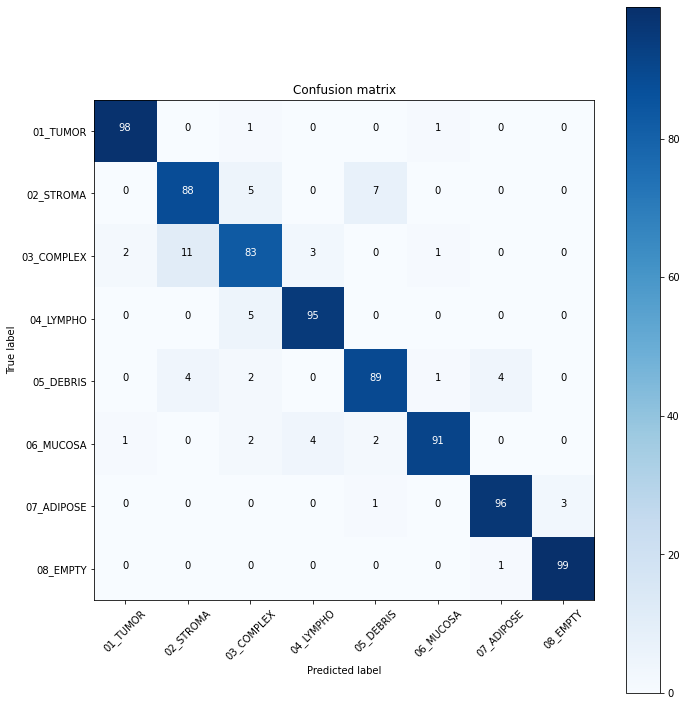
y_preds = np.concatenate(y_preds)cm = confusion_matrix(test_df.label_num.values, y_preds)
plot_confusion_matrix(cm, label_num)Confusion matrix, without normalization: [[98 0 1 0 0 1 0 0] [ 0 88 5 0 7 0 0 0] [ 2 11 83 3 0 1 0 0] [ 0 0 5 95 0 0 0 0] [ 0 4 2 0 89 1 4 0] [ 1 0 2 4 2 91 0 0] [ 0 0 0 0 1 0 96 3] [ 0 0 0 0 0 0 1 99]]
print(classification_report(
  test_df.label_num.values,
  y_preds,
  target_names=list(label_num.keys())
))precision recall f1-score support 01_TUMOR 0.97 0.98 0.98 100 02_STROMA 0.85 0.88 0.87 100 03_COMPLEX 0.85 0.83 0.84 100 04_LYMPHO 0.93 0.95 0.94 100 05_DEBRIS 0.90 0.89 0.89 100 06_MUCOSA 0.97 0.91 0.94 100 07_ADIPOSE 0.95 0.96 0.96 100 08_EMPTY 0.97 0.99 0.98 100 accuracy 0.92 800
Conclusion
We trained ResNet-50 for 15 epochs achieving 92% accuracy on the test set. Tumor and Empty classes are the most recognisable (F1 = 0.98). The most confusable label is Complex, which likely represents combinations of other tissue types.