Time Series Forecasting: LSTM-based model for metro traffic prediction (PyTorch)

This tutorial contains brief overview of statistical and machine learning methods for time series forecasting, experiments and comparative analysis of Long short-term memory (LSTM) based architectures for solving above mentioned problem. Single layer, two layer and bidirectional single layer LSTM cases are considered. Metro Interstate Traffic Volume Data Set from UCI Machine Learning Repository and PyTorch deep learning framework are used for analysis.

• • •

Time series forecasting methods overview

A time series is a set of observations, each one is being recorded at the specific time $t$ . It can be weather observations, for example, a records of the temperature for a month, it can be observations of currency quotes during the day or any other process aggregated by time. Time series forecasting can be determened as the act of predicting the future by understanding the past. The model for forecasting can rely on one variable and this is a univariate case or when more than one variable taken into consideration it will be multivariate case.

Stochastic Linear Models:

Autoregressive (AR);
Moving Average (MA);
Autoregressive Moving Average (ARMA);
Autoregressive Integrated Moving Average (ARIMA);
Seasonal ARIMA (SARIMA).

For above family of models, the stationarity condition must be satisfied. Loosely speaking, a stochastic process is stationary, if its statistical properties do not change with time.

Stochastic Non-Linear Models:

nonlinear autoregressive exogenous models (NARX);
autoregressive conditional heteroskedasticity (ARCH);
generalized autoregressive conditional heteroskedasticity (GARCH).

Machine Learning Models

Hidden Markov Model;
Least-square SVM (LS-SVM);
Dynamic Least-square SVM (DLS-SVM);
Feed Forward Network (FNN);
Time Lagged Neural Network (TLNN);
Seasonal Artificial Neural Network (SANN);
Recurrent Neural Networks (RNN).

Dataset

We will use Metro Interstate Traffic Volume Data Set from UC Irvine Machine Learning Repository, which contains large number of datasets for various tasks in machine learning. We will investigate how weather and holiday features influence the metro traffic in US.

Attribute Information:

holiday — Categorical US National holidays plus regional holiday, Minnesota State;
temp — Numeric, average temp in kelvin;
rain_1h — Numeric, amount in mm of rain that occurred in the hour;
snow_1h — Numeric, amount in mm of snow that occurred in the hour;
clouds_all — Numeric, percentage of cloud cover;
weather_main — Categorical, short textual description of the current weather;
weather_description — Categorical, longer textual description of the current weather;
date_time — DateTime, hour of the data collected in local CST time;
traffic_volume — Numeric, hourly I-94 ATR 301 reported westbound traffic volume.

Our target variable will be traffic_volume. Here we will consider multivariate multi-step prediction case with LSTM-based recurrent neural network architecture.

Metro Traffic Prediction using LSTM-based recurrent neural network

I used Google Colab Notebooks to calculate experiments. Here, for convenience, I mounted my Google Drive where I stored the files.

Out [1]:

Mounted at /content/drive

Exploratory Data Analysis (EDA) and Scaling

Сategorical features: holiday, weather_main, weather_description.
Continious features: temp, rain_1h, show_1h, clouds_all.
Target variable: traffic_volume

Checking for Nan values

Here I take into consideration two categorical variables, such as holiday and weather_main and then one-hot encode them.

Here we can see outliers in temp variable, lets filter outliers with Interquartile range (IQR) method

Normalizing the features

Preparing training dataset and Visualizations

Here we will consider multiple future points prediction case given a past history.

LSTM Time Series Predictor Model

For more efficient storing of long sequences, here I chose the LSTM architecture. LSTM layer consists from cells which is shown below. Two vectors are inputs to the LSTM-cell: the new input vector from the data $x_t$ and the vector of the hidden state $h_{t-1}$ , which is obtained from the hidden state of this cell in the previous time step.

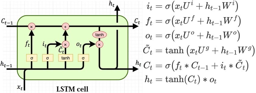
Where:

$i_t$ - input gate
$f_t$ - forget gate
$o_t$ - output gate
$\tilde{C_t}$ - new candidate cell state
$C_t$ - cell state
$h_t$ - block output

Train and Evaluate Helping Functions

1-Layer LSTM model

Test

2-Layer LSTM

Test

Bidirectional 1-Layer LSTM

Test

Experimental results on val data

Model	Best MSE loss
1-layer LSTM	0.66802
2-layer LSTM	0.66578
Bidirectional 1-layer LSTM	0.66894

Summary

At the first glance, all three models based on LSTM showed approximately the same results, so you can choose a single-layer LSTM without loss of quality. In cases where computational efficiency is a crucial part you may chose GRU model, which has less parameters to optimize than LSTM model.

The ways you can improve existing deep learning model:

Work on data cleanliness, look for essential features, which are strongly related to the target variable
Manual and automatic feature engineering
Optimization of hyperparameters (length of hidden state vector, batch size, number of epochs, learning rate, number of layers)
Try different optimization algorithm
Try different loss function which will be differentiable and adequate to task you're solving
Use ensembles of prediction vectors